Quantum Dynamics: Analytical & Computational Solutions in Python

Master time evolution in quantum mechanics. Learn to solve the harmonic oscillator and double-well tunneling using both analytical math and computational Python.
Quantum Physics
Computational Physics
Python
Advanced
Harmonic Oscillator

You Will Learn

S.No. Analytical Methods Computational Methods
1 Operator Algebra (\(\hat{a}\), \(\hat{a}^\dagger\)) Libraries: Python, NumPy, SciPy, Matplotlib
2 Hermite Polynomials & Special Functions Matrix Diagonalization
3 WKB Approximation Finite Difference Method (FDM)
4 Eigenfunction Expansion Shooting Method
5 Gaussian Integrals & Error Functions Runge-Kutta Methods (RK4)
6 Dirac Notation Manipulation Crank-Nicolson Scheme
7 Fourier Transforms (Momentum Space) Root-Finding (Newton-Raphson, Bisection)

Problem 1: The Truncated Parabola in a Harmonic Oscillator

Problem Statement

Consider a particle of mass \(m\) subject to a one-dimensional quantum harmonic oscillator potential: \[V(x)=\frac{1}{2}m\omega^2x^2\]

At time \(t=0\), the particle is prepared in the initial state: \[\psi(x,0)=\begin{cases}N(A-Bx^2)&\text{for }x^2\le\frac{A}{B}\\0&\text{for }x^2>\frac{A}{B}\end{cases}\]

where \(A\) and \(B\) are positive real constants, and \(N\) is the normalization constant.

Tasks
  1. Determine the normalization constant \(N\).
  2. Calculate the probability of finding the particle in the energy eigenstates \(E_n\).
  3. Write down the expression for the time-evolved wave function \(\psi(x,t)\).

Solution & Dynamics

Analytical Solution

1. Finding the Normalization Constant \(N\)

To normalize the wavefunction \(\psi(x,0)\), we require the integral of its probability density over all space to equal \(1\): \[\int_{-\infty}^{\infty} |\psi(x,0)|^2 dx = 1\]

Since the wavefunction is zero for \(x^2 > A/B\), the integration limits are restricted to \(\pm \sqrt{A/B}\): \[\int_{-\sqrt{A/B}}^{\sqrt{A/B}} N^2 (A - Bx^2)^2 dx = 1\]

We expand the integrand and use the symmetry (even function) to double the integral from \(0\) to \(\sqrt{A/B}\): \[2N^2 \int_{0}^{\sqrt{A/B}} (A^2 - 2ABx^2 + B^2x^4) dx = 1\]

Integrating term-by-term: \[2N^2 \left[ A^2x - \frac{2}{3}ABx^3 + \frac{1}{5}B^2x^5 \right]_0^{\sqrt{A/B}} = 1\]

Substituting the upper limit \(x_0 = \sqrt{A/B}\): \[2N^2 \left( A^2\sqrt{\frac{A}{B}} - \frac{2}{3}AB\left(\frac{A}{B}\right)^{3/2} + \frac{1}{5}B^2\left(\frac{A}{B}\right)^{5/2} \right) = 1\] \[2N^2 \frac{A^{5/2}}{B^{1/2}} \left( 1 - \frac{2}{3} + \frac{1}{5} \right) = 1\] \[2N^2 \frac{A^{5/2}}{B^{1/2}} \left( \frac{15 - 10 + 3}{15} \right) = 1 \implies N^2 \left( \frac{16 A^{5/2}}{15 B^{1/2}} \right) = 1\]

Solving for \(N\) (choosing the positive root): \[\boxed{N = \frac{\sqrt{15} B^{1/4}}{4 A^{5/4}}}\]

2. Overlap Coefficients & Probabilities

The probability \(P_n\) of measuring the energy eigenvalue \(E_n = (n + \frac{1}{2})\hbar\omega\) is given by \(P_n = |c_n|^2\), where \(c_n\) is the overlap integral of the initial state with the \(n\)-th eigenstate: \[c_n = \int_{-\infty}^{\infty} \psi_n(x) \psi(x,0) dx\]

The normalized eigenstates of the 1D quantum harmonic oscillator are: \[\psi_n(x) = \left(\frac{\alpha^2}{\pi}\right)^{1/4} \frac{1}{\sqrt{2^n n!}} H_n(\alpha x) e^{-\frac{1}{2}\alpha^2 x^2}\] where \(\alpha = \sqrt{m\omega/\hbar}\).

  • Parity (Symmetry) Argument: The initial wavefunction \(\psi(x,0)\) is symmetric about the origin (even parity). The \(n\)-th eigenfunction \(\psi_n(x)\) has the parity of \((-1)^n\).
    • For odd \(n\), \(\psi_n(x)\) is an odd function. The product of an even and an odd function is odd, making the integral over the symmetric interval \([-x_0, x_0]\) vanish: \[\boxed{c_n = 0 \quad \text{for odd } n \implies P_n = 0}\]
    • For even \(n\), \(\psi_n(x)\) is an even function, and the overlap is non-zero: \[c_n = 2 N \left(\frac{\alpha^2}{\pi}\right)^{1/4} \frac{1}{\sqrt{2^n n!}} \int_{0}^{\sqrt{A/B}} (A - Bx^2) H_n(\alpha x) e^{-\frac{1}{2}\alpha^2 x^2} dx\] Evaluating this integral analytically for general even \(n\) yields complex expressions containing special functions. Thus, we compute it numerically using Simpson’s integration rule.
3. Time Evolution

The time-evolved wavefunction \(\psi(x,t)\) is constructed using the expansion: \[\psi(x,t) = \sum_{n=0}^{\infty} c_n \psi_n(x) e^{-i E_n t / \hbar}\]

Substituting \(c_n = 0\) for odd \(n\), this simplifies to a summation over even eigenstates: \[\boxed{\psi(x,t) = \sum_{k=0}^{\infty} c_{2k} \psi_{2k}(x) e^{-i E_{2k} t / \hbar}}\] where \(E_{2k} = \left(2k + \frac{1}{2}\right)\hbar\omega\).


Computational Solution

Below is the Python implementation that solves the normalization, computes the coefficients, plots the 2-panel physical dashboard, and renders the live interactive time-evolution of the wavefunction. We hardcode physical parameters representing an electron in an optical harmonic potential:

Code
import numpy as np
import matplotlib.pyplot as plt
import matplotlib.animation as animation
from scipy.integrate import simpson
from scipy.special import eval_hermite, factorial
from IPython.display import HTML

# --- 1. Physical Parameters (SI Units) ---
A = 1.0
B = 1.38e18
m = 9.1e-31         # kg (electron mass)
omega = 1e15        # rad/s (angular frequency)
t_eval = 1.57e-15   # seconds (t = T/4)
n_max = 12          # number of eigenstates
hbar = 1.0545718e-34 # J.s

# Analytical Normalization Constant
N = (np.sqrt(15) * (B**0.25)) / (4 * (A**1.25))
# Natural length scale
l = np.sqrt(hbar / (m * omega))

# Spatial grid (dimensionless u = x/l)
x_max = 8 * l
x = np.linspace(-x_max, x_max, 5000)
dx = x[1] - x[0]
u = x / l

# Initial State
psi0 = np.zeros_like(x)
mask = x**2 <= (A / B)
psi0[mask] = N * (A - B * x[mask]**2)

# --- 2. Eigenfunction Coefficients ---
alpha = np.sqrt(m * omega / hbar)

def psi_n(n, x):
    norm = ((alpha**2 / np.pi)**0.25) / np.sqrt((2.0**n) * factorial(n))
    Hn = eval_hermite(n, alpha * x)
    return norm * Hn * np.exp(-0.5 * (alpha * x)**2)

coefficients = []
probabilities = []
energies = []

for n in range(n_max):
    psiN = psi_n(n, x)
    cn = simpson(psiN * psi0, x)
    Pn = np.abs(cn)**2
    En = (n + 0.5) * hbar * omega
    coefficients.append(cn)
    probabilities.append(Pn)
    energies.append(En)

coefficients = np.array(coefficients)
probabilities = np.array(probabilities)
energies = np.array(energies)

# Time Evolution at specified t_eval
psi_t = np.zeros_like(x, dtype=complex)
for n in range(n_max):
    phase = np.exp(-1j * energies[n] * t_eval / hbar)
    psi_t += coefficients[n] * psi_n(n, x) * phase

# --- 3. 2-Panel Plotting ---
phi0_scaled = psi0 * np.sqrt(l)
phit_scaled = psi_t * np.sqrt(l)
prob0_scaled = np.abs(phi0_scaled)**2
probt_scaled = np.abs(phit_scaled)**2

fig, (ax1, ax2) = plt.subplots(1, 2, figsize=(11, 5), layout="constrained")
plot_colors = {
    'potential': '#64748b', 'initial_wf': '#94a3b8', 'evolved_wf_real': '#3b82f6',
    'evolved_wf_imag': '#f43f5e', 'evolved_prob': '#8b5cf6', 'grid': '#e2e8f0'
}

# Panel 1: Wavefunctions and Well
V_u = 0.5 * u**2
ax1.plot(u, V_u, color=plot_colors['potential'], ls='--', lw=1.5, label='Potential $V(u) = 0.5 u^2$')
ax1.fill_between(u, prob0_scaled, color=plot_colors['initial_wf'], alpha=0.15, label=r'$|\psi(u,0)|^2$ (Initial)')
ax1.plot(u, np.real(phit_scaled), color=plot_colors['evolved_wf_real'], lw=1.5, label=r'$\mathrm{Re}[\psi(u,t)]$')
ax1.plot(u, np.imag(phit_scaled), color=plot_colors['evolved_wf_imag'], lw=1.5, ls=':', label=r'$\mathrm{Im}[\psi(u,t)]$')
ax1.fill_between(u, probt_scaled, color=plot_colors['evolved_prob'], alpha=0.25, label=r'$|\psi(u,t)|^2$ (Evolved)')
ax1.set_xlim(-5, 5)
ax1.set_ylim(-1.2, 1.8)
ax1.set_title("Wavefunction Dynamics & Potential Well", fontsize=11, fontweight='semibold')
ax1.set_xlabel(r"Dimensionless Coordinate $u = x/l$")
ax1.set_ylabel("Amplitude / Probability Density")
ax1.grid(True, linestyle=':', alpha=0.6, color=plot_colors['grid'])
ax1.legend(loc='upper right', framealpha=0.9)
ax1.spines['top'].set_visible(False)
ax1.spines['right'].set_visible(False)

# Panel 2: Energy Spectrum
bars = ax2.bar(np.arange(n_max), probabilities, color=plot_colors['evolved_prob'], edgecolor='#7c3aed', alpha=0.8, width=0.5)
ax2.set_title("Energy Spectrum $|c_n|^2$", fontsize=11, fontweight='semibold')
ax2.set_xlabel("Quantum Number $n$")
ax2.set_ylabel("Probability $P_n$")
ax2.set_xticks(np.arange(n_max))
ax2.grid(True, linestyle=':', alpha=0.6, color=plot_colors['grid'], axis='y')
ax2.spines['top'].set_visible(False)
ax2.spines['right'].set_visible(False)

for bar in bars:
    height = bar.get_height()
    if height > 0.005:
        ax2.text(bar.get_x() + bar.get_width()/2.0, height + 0.01, f"{height:.3f}", ha='center', va='bottom', fontsize=8)

plt.show()

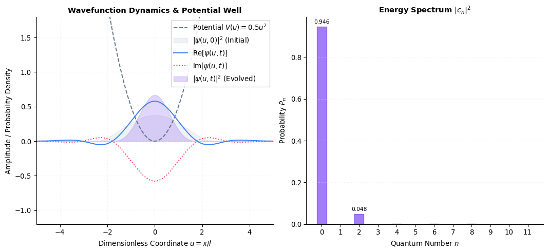
Left: Potential well V(u) along with the initial wavefunction (shaded gray) and time-evolved wavefunction (colored lines) at t = T/4. Right: Energy eigenstate probability spectrum.
Live Time Evolution Animation

The code below compiles a continuous time-evolution of the wavefunction over two periods (\(t \in [0, 2T]\)). The engine will render it inline as an interactive JavaScript player:

Code
fig_anim, ax_anim = plt.subplots(figsize=(7, 4.5), layout="constrained")
ax_anim.set_xlim(-5, 5)
ax_anim.set_ylim(-1.2, 1.8)
ax_anim.set_title(r"Wavefunction Time Evolution $\psi(u, t)$", fontsize=11, fontweight='semibold')
ax_anim.set_xlabel(r"Dimensionless Coordinate $u = x/l$")
ax_anim.set_ylabel("Amplitude / Probability Density")
ax_anim.grid(True, linestyle=':', alpha=0.6, color=plot_colors['grid'])
ax_anim.spines['top'].set_visible(False)
ax_anim.spines['right'].set_visible(False)

# Background Potential Well
ax_anim.plot(u, V_u, color=plot_colors['potential'], ls='--', lw=1.5, label='Potential $V(u)$')

line_prob, = ax_anim.plot([], [], color=plot_colors['evolved_prob'], lw=2.2, label=r'$|\psi(u, t)|^2$')
line_real, = ax_anim.plot([], [], color=plot_colors['evolved_wf_real'], lw=1.3, label=r'$\mathrm{Re}[\psi(u, t)]$')
line_imag, = ax_anim.plot([], [], color=plot_colors['evolved_wf_imag'], lw=1.3, ls=':', label=r'$\mathrm{Im}[\psi(u, t)]$')
fill_coll = [ax_anim.fill_between([], [], color=plot_colors['evolved_prob'], alpha=0.15)]

time_text = ax_anim.text(
    0.05, 0.90, '', transform=ax_anim.transAxes, fontsize=9, fontweight='bold',
    bbox=dict(facecolor='white', alpha=0.9, edgecolor='#cbd5e1', boxstyle='round,pad=0.4')
)
ax_anim.legend(loc='upper right')

# Setup animation details (60 frames over 2 complete periods)
T_period = 2 * np.pi / omega
num_frames = 60
t_fracs = np.linspace(0, 2, num_frames)

def init():
    line_prob.set_data([], [])
    line_real.set_data([], [])
    line_imag.set_data([], [])
    time_text.set_text('')
    return line_prob, line_real, line_imag, time_text

def update(frame):
    t_frac = t_fracs[frame]
    t_val = t_frac * T_period
    
    # Calculate time-evolved wavefunction
    psi_t_anim = np.zeros_like(x, dtype=complex)
    for n in range(n_max):
        phase = np.exp(-1j * (n + 0.5) * omega * t_val)
        psi_t_anim += coefficients[n] * psi_n(n, x) * phase
        
    phi_t_anim = psi_t_anim * np.sqrt(l)
    prob_t_anim = np.abs(phi_t_anim)**2
    real_t_anim = np.real(phi_t_anim)
    imag_t_anim = np.imag(phi_t_anim)
    
    line_prob.set_data(u, prob_t_anim)
    line_real.set_data(u, real_t_anim)
    line_imag.set_data(u, imag_t_anim)
    
    fill_coll[0].remove()
    fill_coll[0] = ax_anim.fill_between(u, prob_t_anim, color=plot_colors['evolved_prob'], alpha=0.15)
    time_text.set_text(rf"$t = {t_frac:.2f}\,T$")
    return line_prob, line_real, line_imag, time_text

ani = animation.FuncAnimation(
    fig_anim, update, frames=num_frames, init_func=init, blit=False, interval=70
)

# Render Javascript player and suppress the static canvas output
html_str = ani.to_jshtml()
custom_css = """
.anim-buttons button[title="Decrease speed"],
.anim-buttons button[title="First frame"],
.anim-buttons button[title="Previous frame"],
.anim-buttons button[title="Play backwards"],
.anim-buttons button[title="Next frame"],
.anim-buttons button[title="Last frame"],
.anim-buttons button[title="Increase speed"] {
    display: none !important;
}
.anim-state input[type="radio"] {
    margin-right: 6px !important;
}
.anim-state label {
    margin-right: 20px !important;
}
"""
html_str = html_str.replace("</style>", f"{custom_css}\n</style>")
js_player = HTML(html_str)
plt.close(fig_anim)
js_player

Problem 2: The Shifted and Squeezed Gaussian

A particle of mass \(m\) in a harmonic oscillator potential \(V(x)=\frac{1}{2}m\omega^2x^2\) is initially prepared in a Gaussian wave packet given by: \[\psi(x,0)=Ne^{-\frac{(x-x_0)^2}{2a^2}}\] where \(x_0\) is an initial spatial shift, \(a\) is the initial width of the wave packet, and \(a\neq\sqrt{\hbar/m\omega}\) (which is the natural width of the oscillator ground state).

Tasks
  1. Determine the time evolution of the wave packet, \(\psi(x,t)\).
  2. Calculate the expectation values of position \(\langle x\rangle(t)\) and momentum \(\langle p\rangle(t)\).
  3. Determine the uncertainty in position \(\Delta x(t)\) and show how the wave packet width oscillates or “breathes” over time.

Solution & Dynamics

Analytical Solution

1. Time Evolution of Expectation Values

Using Ehrenfest’s Theorem for a particle in a harmonic oscillator potential \(V(x) = \frac{1}{2} m \omega^2 x^2\), the expectation values obey classical equations of motion: \[ \frac{d\langle x \rangle}{dt} = \frac{\langle p \rangle}{m}, \quad \frac{d\langle p \rangle}{dt} = -m \omega^2 \langle x \rangle \] Solving these coupled differential equations with initial conditions \(\langle x \rangle(0) = x_0\) and \(\langle p \rangle(0) = 0\) yields: \[ \boxed{ \langle x \rangle(t) = x_0 \cos(\omega t) } \] \[ \boxed{ \langle p \rangle(t) = -m \omega x_0 \sin(\omega t) } \] The center of the wave packet oscillates harmonically with frequency \(\omega\).

2. Position Uncertainty and “Breathing”

For a Gaussian wave packet, the uncertainty in position \(\Delta x(t)\) depends on its initial width \(a\). If the initial width differs from the natural width of the oscillator ground state \(l = \sqrt{\hbar / m \omega}\), the state is “squeezed”. The time evolution of the variance is given by: \[ (\Delta x(t))^2 = \frac{a^2}{2} \cos^2(\omega t) + \frac{\hbar^2}{2 m^2 \omega^2 a^2} \sin^2(\omega t) \] Taking the square root gives the position uncertainty: \[ \boxed{ \Delta x(t) = \frac{a}{\sqrt{2}} \sqrt{ \cos^2(\omega t) + \left( \frac{l^2}{a^2} \right)^2 \sin^2(\omega t) } } \] This shows that the width of the wave packet oscillates (or “breathes”) with a frequency \(2\omega\). If \(a = l\), the width remains constant \(\Delta x(t) = l/\sqrt{2}\) (coherent state).

Computational Solution

We will compute the evolution numerically by expanding the Gaussian in the basis of harmonic oscillator eigenstates.

Code
# --- 1. Physical Parameters ---
x0 = 3.0 * l        # initial shift
a = 0.5 * l         # squeezed width (narrower than ground state)
n_max2 = 40         # number of eigenstates for expansion
T_period = 2 * np.pi / omega

# Initial State
N_g = (np.pi * a**2)**(-0.25)
psi0_g = N_g * np.exp(-0.5 * ((x - x0)/a)**2)

# --- 2. Eigenfunction Coefficients ---
coefficients_g = []
for n in range(n_max2):
    psiN = psi_n(n, x)
    cn = simpson(psiN * psi0_g, x)
    coefficients_g.append(cn)
coefficients_g = np.array(coefficients_g)

# Time Evolution function
def get_psi_t_g(t_val):
    psi_t = np.zeros_like(x, dtype=complex)
    for n in range(n_max2):
        En = (n + 0.5) * hbar * omega
        phase = np.exp(-1j * En * t_val / hbar)
        psi_t += coefficients_g[n] * psi_n(n, x) * phase
    return psi_t

# --- 3. 2-Panel Plotting ---
t_half = T_period / 2.0
psi_half = get_psi_t_g(t_half)

fig2, (ax2_1, ax2_2) = plt.subplots(1, 2, figsize=(11, 5), layout="constrained")

# Panel 1: Wavefunctions and Well
ax2_1.plot(u, V_u, color=plot_colors['potential'], ls='--', lw=1.5, label='Potential $V(u)$')
ax2_1.fill_between(u, (np.abs(psi0_g)*np.sqrt(l))**2, color='#3b82f6', alpha=0.3, label=r'$|\psi(u,0)|^2$')
ax2_1.fill_between(u, (np.abs(psi_half)*np.sqrt(l))**2, color='#f43f5e', alpha=0.3, label=r'$|\psi(u,T/2)|^2$')
ax2_1.set_xlim(-6, 6)
ax2_1.set_ylim(-0.2, 2.5)
ax2_1.set_title("Wavepacket Bouncing in Potential", fontsize=11, fontweight='semibold')
ax2_1.set_xlabel(r"Dimensionless Coordinate $u = x/l$")
ax2_1.set_ylabel("Probability Density")
ax2_1.grid(True, linestyle=':', alpha=0.6)
ax2_1.legend(loc='upper center', framealpha=0.9)
ax2_1.spines['top'].set_visible(False)
ax2_1.spines['right'].set_visible(False)

# Panel 2: Expectation Values over Time
t_array = np.linspace(0, 1.5 * T_period, 100)
x_exp_comp, dx_comp = [], []
for t_val in t_array:
    pt = get_psi_t_g(t_val)
    prob_t = np.abs(pt)**2
    x_exp = simpson(x * prob_t, x)
    x2_exp = simpson(x**2 * prob_t, x)
    x_exp_comp.append(x_exp / l)
    dx_comp.append(np.sqrt(x2_exp - x_exp**2) / l)

# Analytical
x_exp_ana = (x0 / l) * np.cos(omega * t_array)
dx_ana = (a / (np.sqrt(2)*l)) * np.sqrt(np.cos(omega*t_array)**2 + (l/a)**4 * np.sin(omega*t_array)**2)

ax2_2.plot(t_array / T_period, x_exp_ana, 'k-', lw=2, label=r'Analytical $\langle x \rangle$')
ax2_2.plot(t_array / T_period, x_exp_comp, 'o', color='#3b82f6', markersize=4, label=r'Comp $\langle x \rangle$')
ax2_2.plot(t_array / T_period, dx_ana, 'k--', lw=2, label=r'Analytical $\Delta x$')
ax2_2.plot(t_array / T_period, dx_comp, 's', color='#f43f5e', markersize=3, label=r'Comp $\Delta x$')
ax2_2.set_title("Observables vs Time", fontsize=11, fontweight='semibold')
ax2_2.set_xlabel("Time $t/T$")
ax2_2.set_ylabel("Dimensionless Units")
ax2_2.grid(True, linestyle=':', alpha=0.6)
ax2_2.legend(loc='upper right')
ax2_2.spines['top'].set_visible(False)
ax2_2.spines['right'].set_visible(False)

plt.show()

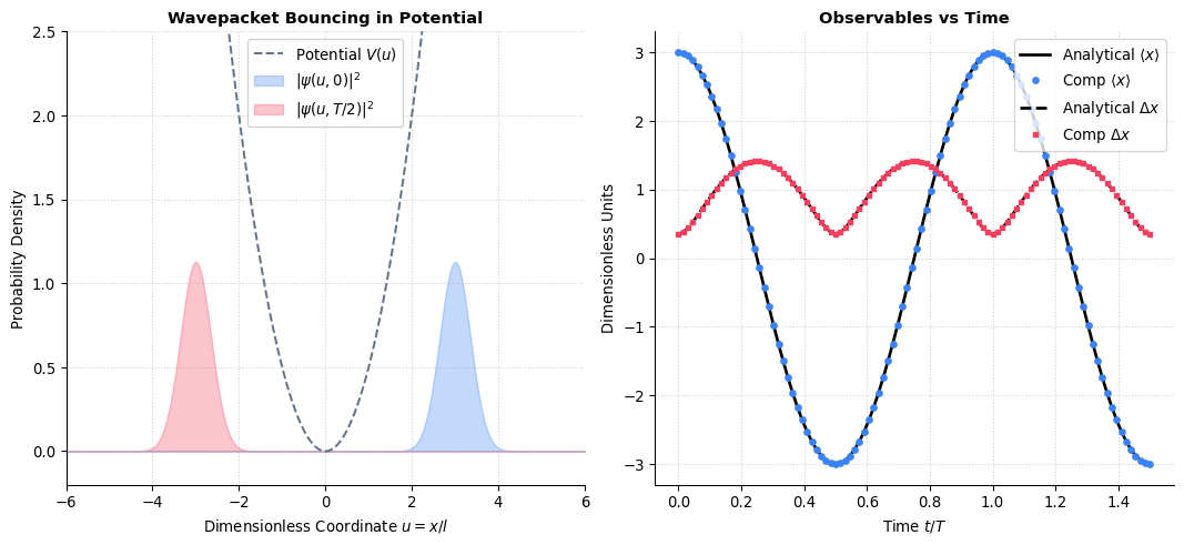
Left: Potential well V(x) along with the initial and half-period wavefunctions. Right: Analytical vs Computational expectation value and position uncertainty.
Live Time Evolution Animation
Code
fig_anim2, ax_anim2 = plt.subplots(figsize=(7, 4.5), layout="constrained")
ax_anim2.set_xlim(-6, 6)
ax_anim2.set_ylim(-0.2, 2.5)
ax_anim2.set_title(r"Squeezed Wavepacket Evolution $|\psi(u, t)|^2$", fontsize=11, fontweight='semibold')
ax_anim2.set_xlabel(r"Dimensionless Coordinate $u = x/l$")
ax_anim2.set_ylabel("Probability Density")
ax_anim2.grid(True, linestyle=':', alpha=0.6, color=plot_colors['grid'])
ax_anim2.spines['top'].set_visible(False)
ax_anim2.spines['right'].set_visible(False)

ax_anim2.plot(u, V_u, color='#64748b', ls='--', lw=1.5, label='Potential $V(u)$')
line_prob2, = ax_anim2.plot([], [], color='#8b5cf6', lw=2.2)
fill_coll2 = [ax_anim2.fill_between([], [], color='#8b5cf6', alpha=0.3)]
time_text2 = ax_anim2.text(0.05, 0.90, '', transform=ax_anim2.transAxes, fontsize=9, fontweight='bold', bbox=dict(facecolor='white', alpha=0.9, edgecolor='#cbd5e1', boxstyle='round,pad=0.4'))

num_frames2 = 60
t_fracs2 = np.linspace(0, 2, num_frames2)

def init2():
    line_prob2.set_data([], [])
    time_text2.set_text('')
    return line_prob2, time_text2

def update2(frame):
    t_frac = t_fracs2[frame]
    t_val = t_frac * T_period
    psi_t = get_psi_t_g(t_val)
    prob_t_anim = (np.abs(psi_t)*np.sqrt(l))**2
    
    line_prob2.set_data(u, prob_t_anim)
    fill_coll2[0].remove()
    fill_coll2[0] = ax_anim2.fill_between(u, prob_t_anim, color='#8b5cf6', alpha=0.3)
    time_text2.set_text(rf"$t = {t_frac:.2f}\,T$")
    return line_prob2, time_text2

ani2 = animation.FuncAnimation(fig_anim2, update2, frames=num_frames2, init_func=init2, blit=False, interval=70)
html_str2 = ani2.to_jshtml().replace("</style>", f"{custom_css}\n</style>")
js_player2 = HTML(html_str2)
plt.close(fig_anim2)
js_player2

Problem 3: Tunneling in the Quartic Double Well

A particle of mass \(m\) moves in a one-dimensional quartic double-well potential described by: \[V(x)=-\frac{1}{2}\alpha x^2+\beta x^4\] where \(\alpha\) and \(\beta\) are positive constants.

Tasks
  1. Find the exact energy eigenvalues for the ground state (\(E_0\)) and the first excited state (\(E_1\)) using computational methods.
  2. Calculate the energy splitting \(\Delta E=E_1-E_0\).
  3. Determine the tunneling time \(\tau\propto\frac{\hbar}{\Delta E}\) for a particle initially localized in the right well to tunnel to the left well.

Solution & Dynamics

Analytical Solution

For a quartic double-well potential \(V(x)=-\frac{1}{2}\alpha x^2+\beta x^4\), there are two minima at \(x_{min} = \pm \sqrt{\alpha/4\beta}\).

1. Degeneracy and Splitting

When the barrier between the wells is high, the lowest two energy levels are nearly degenerate. The true ground state \(\psi_0(x)\) is symmetric, while the first excited state \(\psi_1(x)\) is antisymmetric: \[ \psi_0(x) \approx \frac{1}{\sqrt{2}} (\phi_L(x) + \phi_R(x)) \] \[ \psi_1(x) \approx \frac{1}{\sqrt{2}} (\phi_L(x) - \phi_R(x)) \] where \(\phi_L\) and \(\phi_R\) are states localized in the left and right wells, respectively. The energy splitting \(\Delta E = E_1 - E_0\) is small and determines the tunneling dynamics.

2. Tunneling Time

If a particle is initially localized entirely in the right well, the initial state is a superposition: \[ \Psi(x,0) = \phi_R(x) = \frac{1}{\sqrt{2}} (\psi_0(x) - \psi_1(x)) \] The time evolution introduces a relative phase between the eigenstates: \[ \Psi(x,t) = \frac{1}{\sqrt{2}} \left( \psi_0(x) e^{-i E_0 t / \hbar} - \psi_1(x) e^{-i E_1 t / \hbar} \right) \] The particle completely tunnels to the left well when the relative phase reaches \(\pi\). This occurs at the tunneling time \(\tau\): \[ \frac{(E_1 - E_0)\tau}{\hbar} = \pi \implies \boxed{ \tau = \frac{\pi \hbar}{\Delta E} } \]

Computational Solution

To find the exact eigenvalues and eigenfunctions, we use the Finite Difference Method (FDM) to discretize the Schrödinger equation and turn it into a matrix eigenvalue problem (Hamiltonian diagonalization).

Code
from scipy.sparse import diags
from scipy.sparse.linalg import eigsh

# --- 1. Physical Parameters ---
hbar_dw = 1.0
m_dw = 1.0
alpha_dw = 4.0
beta_dw = 0.5

# Spatial grid for Finite Difference
N_grid = 1000
x_dw = np.linspace(-4, 4, N_grid)
dx_dw = x_dw[1] - x_dw[0]

# Double Well Potential
V_dw = -0.5 * alpha_dw * x_dw**2 + beta_dw * x_dw**4

# --- 2. Matrix Diagonalization (FDM) ---
# Kinetic energy matrix (second derivative)
diag_main = 2.0 * np.ones(N_grid) / (dx_dw**2)
diag_off = -1.0 * np.ones(N_grid - 1) / (dx_dw**2)
T_mat = (hbar_dw**2 / (2 * m_dw)) * diags([diag_off, diag_main, diag_off], [-1, 0, 1])

# Potential energy matrix
V_mat = diags(V_dw, 0)

# Hamiltonian
H_mat = T_mat + V_mat

# Solve for smallest algebraic eigenvalues
eigenvalues, eigenvectors = eigsh(H_mat, k=6, which='SM')

E0, E1 = eigenvalues[0], eigenvalues[1]
psi0_dw = eigenvectors[:, 0] / np.sqrt(dx_dw) # Normalize
psi1_dw = eigenvectors[:, 1] / np.sqrt(dx_dw)

# Fix signs to be consistent
if psi0_dw[N_grid//2] < 0: psi0_dw *= -1
if psi1_dw[N_grid//4] < 0: psi1_dw *= -1

delta_E = E1 - E0
tau_tunnel = np.pi * hbar_dw / delta_E

# --- 3. 2-Panel Plotting ---
fig3, (ax3_1, ax3_2) = plt.subplots(1, 2, figsize=(11, 5), layout="constrained")

# Scale wavefunctions for visualization
scale_factor = 2.0
ax3_1.plot(x_dw, V_dw, color=plot_colors['potential'], ls='--', lw=1.5, label='Potential $V(x)$')
ax3_1.plot(x_dw, E0 + scale_factor * psi0_dw, color='#3b82f6', lw=1.5, label=f'$E_0$ (Sym)')
ax3_1.plot(x_dw, E1 + scale_factor * psi1_dw, color='#f43f5e', lw=1.5, label=f'$E_1$ (Anti-Sym)')
ax3_1.axhline(E0, color='#3b82f6', ls=':', alpha=0.5)
ax3_1.axhline(E1, color='#f43f5e', ls=':', alpha=0.5)

ax3_1.set_xlim(-3, 3)
ax3_1.set_ylim(-3, 2)
ax3_1.set_title("Quartic Double Well & Eigenstates", fontsize=11, fontweight='semibold')
ax3_1.set_xlabel(r"Coordinate $x$")
ax3_1.set_ylabel("Energy")
ax3_1.grid(True, linestyle=':', alpha=0.6)
ax3_1.legend(loc='lower center', framealpha=0.9)
ax3_1.spines['top'].set_visible(False)
ax3_1.spines['right'].set_visible(False)

# Spectrum
ax3_2.plot(np.zeros_like(eigenvalues), eigenvalues, '_', markersize=40, mew=2, color='#8b5cf6')
ax3_2.text(0.05, E0, f"$E_0 = {E0:.3f}$", va='center')
ax3_2.text(0.05, E1, f"$E_1 = {E1:.3f}$", va='center')
ax3_2.annotate('', xy=(0, E1), xytext=(0, E0), arrowprops=dict(arrowstyle='<->', color='black'))
ax3_2.text(-0.02, (E0+E1)/2, rf"$\Delta E = {delta_E:.4f}$", ha='right', va='center', fontweight='bold')

ax3_2.set_xlim(-0.1, 0.2)
ax3_2.set_ylim(-2.5, eigenvalues[-1] + 1)
ax3_2.set_title("Energy Spectrum", fontsize=11, fontweight='semibold')
ax3_2.set_xticks([])
ax3_2.set_ylabel("Energy")
ax3_2.grid(True, linestyle=':', alpha=0.6, axis='y')
ax3_2.spines['top'].set_visible(False)
ax3_2.spines['right'].set_visible(False)
ax3_2.spines['bottom'].set_visible(False)

plt.show()

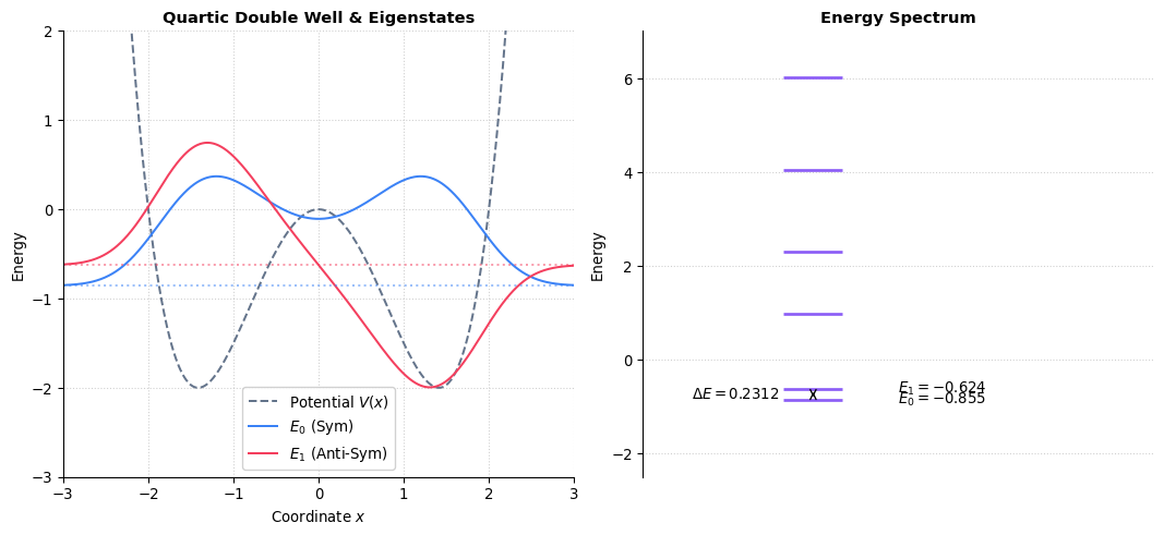
Left: Double well potential and the lowest two eigenstates (symmetric and antisymmetric). Right: Zoomed-in energy spectrum showing the splitting \(\Delta E\).
Live Tunneling Animation
Code
# Initial state localized in the right well
psi_R = (psi0_dw - psi1_dw) / np.sqrt(2)

fig_anim3, ax_anim3 = plt.subplots(figsize=(7, 4.5), layout="constrained")
ax_anim3.set_xlim(-3, 3)
ax_anim3.set_ylim(-3, 1)
ax_anim3.set_title(r"Quantum Tunneling Dynamics", fontsize=11, fontweight='semibold')
ax_anim3.set_xlabel(r"Coordinate $x$")
ax_anim3.set_ylabel("Energy / Probability")
ax_anim3.grid(True, linestyle=':', alpha=0.6, color=plot_colors['grid'])
ax_anim3.spines['top'].set_visible(False)
ax_anim3.spines['right'].set_visible(False)

ax_anim3.plot(x_dw, V_dw, color='#64748b', ls='--', lw=1.5)
line_prob3, = ax_anim3.plot([], [], color='#10b981', lw=2.2, label=r'$|\Psi(x,t)|^2$')
fill_coll3 = [ax_anim3.fill_between([], [], color='#10b981', alpha=0.3)]
time_text3 = ax_anim3.text(0.05, 0.90, '', transform=ax_anim3.transAxes, fontsize=9, fontweight='bold', bbox=dict(facecolor='white', alpha=0.9, edgecolor='#cbd5e1', boxstyle='round,pad=0.4'))
ax_anim3.legend(loc='upper center')

num_frames3 = 80
t_fracs3 = np.linspace(0, 2, num_frames3) # up to 2 * tau

def init3():
    line_prob3.set_data([], [])
    time_text3.set_text('')
    return line_prob3, time_text3

def update3(frame):
    t_frac = t_fracs3[frame]
    t_val = t_frac * tau_tunnel
    
    # Time evolution
    psi_t = (psi0_dw * np.exp(-1j * E0 * t_val / hbar_dw) - 
             psi1_dw * np.exp(-1j * E1 * t_val / hbar_dw)) / np.sqrt(2)
    prob_t = np.abs(psi_t)**2
    
    # Scale and shift to overlay on potential (visual purposes)
    viz_scale = 1.5
    prob_vis = (E0+E1)/2.0 + viz_scale * prob_t
    
    line_prob3.set_data(x_dw, prob_vis)
    fill_coll3[0].remove()
    fill_coll3[0] = ax_anim3.fill_between(x_dw, (E0+E1)/2.0, prob_vis, color='#10b981', alpha=0.3)
    time_text3.set_text(rf"$t = {t_frac:.2f}\,\tau$")
    return line_prob3, time_text3

ani3 = animation.FuncAnimation(fig_anim3, update3, frames=num_frames3, init_func=init3, blit=False, interval=70)
html_str3 = ani3.to_jshtml().replace("</style>", f"{custom_css}\n</style>")
js_player3 = HTML(html_str3)
plt.close(fig_anim3)
js_player3