Computational Quantum Mechanics: Infinite Potential Well
Solving the infinite potential well problem using both analytical and computational methods in Python. This project explores normalization, quantum measurements, expectation values, and time evolution of superposed quantum states.
Quantum Mechanics
Computational Physics
Python
Infinite Potential Well
Author
Aditya Kumar
PublishedMay 25, 2026
Copied!
Problem Statement
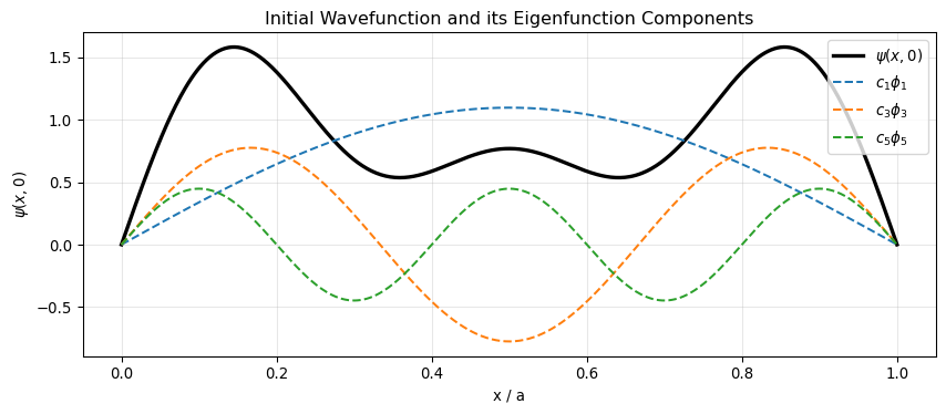
A particle of mass \(m\) moves freely inside a one-dimensional infinite potential well of length \(a\). The potential is:
\[
V(x) = \begin{cases} 0 & 0 \leq x \leq a \\ \infty & \text{otherwise} \end{cases}
\]
This shows that the probability density breathes and shifts in time — the quantum state is alive even though the energy probabilities never change.
The characteristic oscillation period between levels \(m\) and \(n\) is:
\[
T_{mn} = \frac{2\pi\hbar}{|E_m - E_n|}
\]
Computational Solution — Time Evolution Visualisation
Explore different times
Change the value of t_in_T1 below to see \(|\psi(x,t)|^2\) at different moments. The value is in units of \(T_1 = 2\pi\hbar/E_1\).
Code
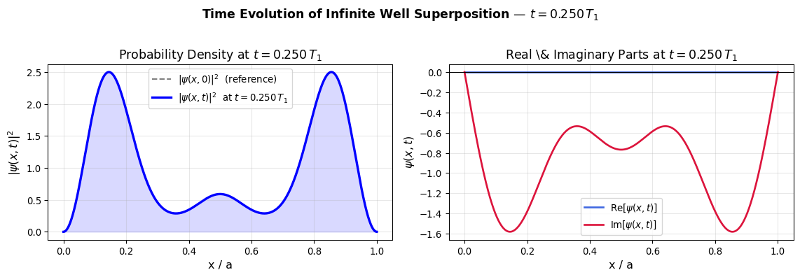
# --- Parameters ---E1 = (np.pi**2* hbar**2) / (2* m * a**2)T1 =2* np.pi * hbar / E1 # Natural period of ground statedef phi_n(n, x):return np.sqrt(2/a) * np.sin(n * np.pi * x / a)def psi_t(x, t):"""Full time-dependent wavefunction (complex).""" c1 = np.sqrt(3/5) c3 = np.sqrt(3/10) c5 =1/ np.sqrt(10)return (c1 * phi_n(1, x) * np.exp(-1j* E1 * t / hbar)+ c3 * phi_n(3, x) * np.exp(-1j*9*E1 * t / hbar)+ c5 * phi_n(5, x) * np.exp(-1j*25*E1 * t / hbar))# =========================================================# Change this value to explore different times# =========================================================t_in_T1 =0.25# time in units of T1t = t_in_T1 * T1# =========================================================x = np.linspace(0, a, 1000)Psi_t = psi_t(x, t)prob_t = np.abs(Psi_t)**2prob_0 = np.abs(psi_t(x, 0))**2fig, axes = plt.subplots(1, 2, figsize=(12, 4))# Left: Probability densityax = axes[0]ax.plot(x, prob_0, 'k--', lw=1.5, alpha=0.5, label=r'$|\psi(x,0)|^2$ (reference)')ax.plot(x, prob_t, 'b-', lw=2.5, label=rf'$|\psi(x,t)|^2$ at $t = {t_in_T1:.3f}\,T_1$')ax.fill_between(x, prob_t, alpha=0.15, color='blue')ax.set_xlabel('x / a', fontsize=12)ax.set_ylabel(r'$|\psi(x,t)|^2$', fontsize=12)ax.set_title(rf'Probability Density at $t = {t_in_T1:.3f}\,T_1$', fontsize=13)ax.legend(fontsize=10)ax.grid(alpha=0.3)# Right: Real and imaginary parts of psi(x,t)ax2 = axes[1]ax2.plot(x, np.real(Psi_t), 'royalblue', lw=2, label=r'Re$[\psi(x,t)]$')ax2.plot(x, np.imag(Psi_t), 'crimson', lw=2, label=r'Im$[\psi(x,t)]$')ax2.axhline(0, color='k', lw=0.8)ax2.set_xlabel('x / a', fontsize=12)ax2.set_ylabel(r'$\psi(x,t)$', fontsize=12)ax2.set_title(rf'Real \& Imaginary Parts at $t = {t_in_T1:.3f}\,T_1$', fontsize=13)ax2.legend(fontsize=10)ax2.grid(alpha=0.3)plt.suptitle(rf'Time Evolution of Infinite Well Superposition — $t = {t_in_T1:.3f}\,T_1$', fontsize=13, fontweight='bold', y=1.02)plt.tight_layout()plt.show()
Probability density and real/imaginary parts of the wavefunction at time \(t = 0.25 T_1\).
Code
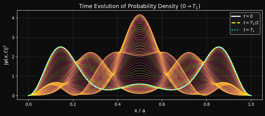
# --- Bonus: Animated time sweep ---# Plots |psi(x,t)|^2 for t from 0 to T1 in 200 steps to show the "breathing"times = np.linspace(0, T1, 200)x = np.linspace(0, a, 500)fig, ax = plt.subplots(figsize=(9, 4))cmap = plt.cm.plasmafor i, t_val inenumerate(times): color = cmap(i /len(times)) ax.plot(x, np.abs(psi_t(x, t_val))**2, color=color, lw=0.8, alpha=0.6)# Overlay t=0 and t=T1/2 prominentlyax.plot(x, np.abs(psi_t(x, 0))**2, 'white', lw=2.5, label=r'$t=0$')ax.plot(x, np.abs(psi_t(x, T1/2))**2, 'yellow', lw=2.5, linestyle='--', label=r'$t=T_1/2$')ax.plot(x, np.abs(psi_t(x, T1))**2, 'cyan', lw=2.5, linestyle=':', label=r'$t=T_1$')ax.set_facecolor('#0d0d0d')fig.patch.set_facecolor('#0d0d0d')ax.tick_params(colors='white')ax.xaxis.label.set_color('white')ax.yaxis.label.set_color('white')ax.title.set_color('white')for spine in ax.spines.values(): spine.set_edgecolor('white')ax.set_xlabel('x / a', fontsize=12)ax.set_ylabel(r'$|\psi(x,t)|^2$', fontsize=12)ax.set_title(r'Time Evolution of Probability Density ($0 \to T_1$)', fontsize=13)ax.legend(fontsize=10, facecolor='#1a1a1a', labelcolor='white')ax.grid(alpha=0.2)plt.tight_layout()plt.show()
Animated sweep showing the time evolution of the probability density from \(t=0\) to \(t=T_1\).
What’s happening in these graphs?
Taking a Snapshot: The first graph acts like a camera taking a picture at a specific time. It shows what the wave looks like at that exact moment.
Time-Lapse Motion: The second graph shows the wave changing over a full time cycle. The different colors show the wave at different times.
The “Breathing” Effect: Notice how the wave sloshes back and forth! This happens because the different simple waves that make up the total wave are vibrating at different speeds, causing them to interfere with each other.
Summary
Part A
Part B
Part C
Goal
Normalize \(\psi\)
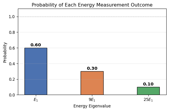
Energy measurements
Time evolution
Key tool
Orthonormality of \(\phi_n\)
Born rule \(P_n = \|c_n\|^2\)
Phase factors \(e^{-iE_n t/\hbar}\)
Result
\(A = \sqrt{6/5}\)
\(\langle E \rangle = 29E_1/5\)
\(\psi(x,t)\) oscillates, \(P_n\) constant
Key Physical Insight
Even though the probability of measuring each energy never changes (energy probabilities are stationary), the probability density \(|\psi(x,t)|^2\)does change in time due to interference between the different eigenstates. The particle’s position is genuinely time-dependent, even in a stationary potential.
References
Zettili, N. Quantum Mechanics: Concepts and Applications, 2nd ed. Wiley, 2009.
Griffiths, D.J. Introduction to Quantum Mechanics, 3rd ed. Cambridge, 2018.
×
Stay Updated!
Join the Physics Voyage newsletter to get the latest articles and courses delivered straight to your inbox.