Quantum Tunneling in a Quartic Double-Well Potential
Why This Problem Matters
The quartic double-well potential is far more than a textbook exercise. It is the simplest system that captures the physics of quantum tunneling — a phenomenon with no classical analogue — and its consequences show up across nearly every branch of modern physics.
Here is why physicists keep coming back to this problem:
- Molecular physics: The ammonia molecule (\(\text{NH}_3\)) has two equivalent configurations (nitrogen above or below the hydrogen plane). The nitrogen atom tunnels between these two positions through a double-well potential. The resulting energy splitting is the operating principle behind the ammonia maser, one of the first masers ever built.
- Condensed matter: Proton transfer in hydrogen bonds, defect migration in crystals, and the dynamics of Josephson junctions in superconducting circuits are all governed by double-well tunneling.
- Quantum computing: Superconducting qubits (transmon, flux qubit) are engineered double-well systems. The tunnel splitting is the qubit frequency. Controlling it is the entire game.
- Quantum field theory: The double-well potential is the prototype for spontaneous symmetry breaking and instanton physics. The tunneling amplitude between degenerate vacua is computed using the same overlap integral we will derive below.
- Chemical physics: Reaction rates in chemistry often involve tunneling through an activation barrier. The Arrhenius law breaks down at low temperatures precisely because of quantum tunneling effects captured by models like this one.
In short, solving the quartic double well teaches you the machinery — overlap integrals, tight-binding models, finite-difference discretization — that you will reuse in far more complex problems.
The Problem
Parameters used throughout this article: \(\hbar = 1\), \(m = 1\), \(\alpha = 4\), \(\beta = 0.5\). These are natural units chosen so that all quantities are of order unity, making the numerics clean and the plots easy to read.
Analytical Solution
We now solve the problem step by step, starting from the shape of the potential and building up to the analytical prediction of the tunnel splitting.
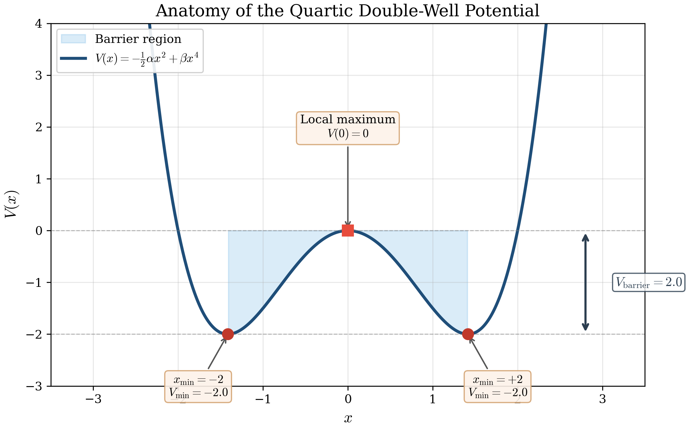
Step 1 — Locating the Minima
To find the extrema of \(V(x)\), we set the first derivative to zero:
\[\frac{dV}{dx} = -\alpha x + 4\beta x^3 = x(-\alpha + 4\beta x^2) = 0\]
This gives three solutions:
- \(x = 0\) — a local maximum (the top of the barrier)
- \(x = \pm\sqrt{\dfrac{\alpha}{4\beta}}\) — two symmetric minima (the bottoms of the wells)
For our parameters:
\[\boxed{x_{\min} = \pm\sqrt{\frac{4}{4 \times 0.5}} = \pm\sqrt{2} \approx \pm 1.414}\]
Step 2 — Barrier Height
The potential at the minima is:
\[V_{\min} = V\!\left(\pm\sqrt{\frac{\alpha}{4\beta}}\right) = -\frac{\alpha^2}{16\beta}\]
The potential at the barrier top is \(V(0) = 0\). Therefore the barrier height above the well floor is:
\[\boxed{V_b = V(0) - V_{\min} = \frac{\alpha^2}{16\beta} = \frac{16}{8} = 2.0}\]
This is the energy a classical particle would need to climb over the hill. A quantum particle, as we shall see, needs far less.
Step 3 — Harmonic Approximation Near Each Minimum
We Taylor-expand \(V(x)\) around \(x_{\min}\) to second order. Writing \(x = x_{\min} + \xi\) (where \(\xi\) is a small displacement):
\[V(x_{\min} + \xi) \approx V_{\min} + \frac{1}{2}V''(x_{\min})\,\xi^2 + \mathcal{O}(\xi^3)\]
Computing the second derivative:
\[V''(x) = -\alpha + 12\beta x^2 \quad\Longrightarrow\quad V''(x_{\min}) = -\alpha + 12\beta\cdot\frac{\alpha}{4\beta} = 2\alpha\]
This is the curvature of a harmonic oscillator with spring constant \(k = 2\alpha\). The effective frequency is:
\[\boxed{\omega_{\text{eff}} = \sqrt{\frac{k}{m}} = \sqrt{\frac{2\alpha}{m}} = \sqrt{8} = 2\sqrt{2} \approx 2.828}\]
Each well, in isolation, behaves like a simple harmonic oscillator with this frequency.
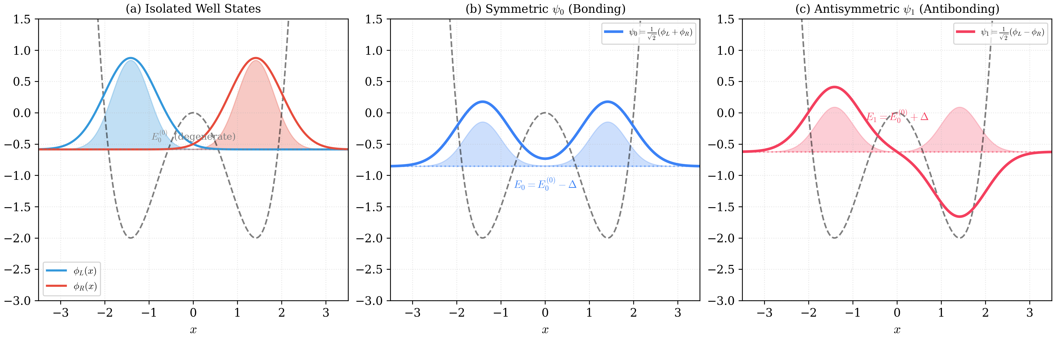
Step 4 — Constructing Localized States
If the barrier were infinitely high, the two wells would be completely isolated. Each would support its own ground-state wavefunction — a Gaussian centred at the respective minimum.
We define:
- \(|\phi_L\rangle\) — the ground state of the left well (centred at \(x = -\sqrt{2}\))
- \(|\phi_R\rangle\) — the ground state of the right well (centred at \(x = +\sqrt{2}\))
Within the harmonic approximation, these are:
\[\phi_{L,R}(x) = \left(\frac{m\omega_{\text{eff}}}{\pi\hbar}\right)^{1/4} \exp\!\left[-\frac{m\omega_{\text{eff}}}{2\hbar}(x \mp \sqrt{2})^2\right]\]
Both states have the same energy:
\[\varepsilon = V_{\min} + \frac{1}{2}\hbar\omega_{\text{eff}} = -2 + \frac{1}{2}(2\sqrt{2}) = -2 + \sqrt{2} \approx -0.586\]
At this stage, the system appears to have a doubly degenerate ground state. But this degeneracy is an artefact of ignoring the barrier region. The next step lifts it.
Step 5 — The Overlap Integral (Tunneling Coupling)
Because the barrier has finite height, the tail of \(\phi_L\) leaks into the right well and vice versa. The two states are not truly orthogonal — they overlap inside the barrier.
We quantify this overlap through the tunneling matrix element:
\[\Delta = -\langle\phi_L|\hat{H}|\phi_R\rangle = -\int_{-\infty}^{\infty} \phi_L^*(x)\,\hat{H}\,\phi_R(x)\,dx\]
What this integral captures:
- The integrand is significant only in the classically forbidden region (under the barrier), where both \(\phi_L\) and \(\phi_R\) have small but nonzero amplitude.
- The operator \(\hat{H}\) includes the kinetic energy term, which measures how rapidly the wavefunction changes — and it changes most rapidly precisely in the barrier region.
- A higher barrier or a wider barrier suppresses the overlap exponentially, making \(\Delta\) smaller.
- A lower or thinner barrier increases the overlap, making \(\Delta\) larger.
The magnitude of \(\Delta\) directly controls how fast the particle tunnels.
Step 6 — Solving the 2 x 2 Eigenvalue Problem
In the basis \(\{|\phi_L\rangle, |\phi_R\rangle\}\), the full Hamiltonian takes the form of a \(2 \times 2\) matrix:
\[\hat{H} = \begin{pmatrix} \varepsilon & -\Delta \\ -\Delta & \varepsilon \end{pmatrix}\]
To find the true energy eigenstates, we solve the secular equation:
\[\det(\hat{H} - E\,\mathbf{I}) = 0\]
\[\det\begin{pmatrix} \varepsilon - E & -\Delta \\ -\Delta & \varepsilon - E \end{pmatrix} = 0\]
\[(\varepsilon - E)^2 - \Delta^2 = 0\]
\[\varepsilon - E = \pm\Delta\]
This yields two distinct energy levels:
\[\boxed{E_0 = \varepsilon - \Delta \qquad (\text{ground state, lower})}\] \[\boxed{E_1 = \varepsilon + \Delta \qquad (\text{first excited state, higher})}\]
Step 7 — The Eigenstates: Bonding and Antibonding
Substituting each eigenvalue back into \(\hat{H}|\psi\rangle = E|\psi\rangle\), we find the corresponding eigenstates:
Ground state (symmetric / bonding): \[|\psi_0\rangle = \frac{1}{\sqrt{2}}\left(|\phi_L\rangle + |\phi_R\rangle\right)\] This state has even parity, no nodes, and its wavefunction has identical positive humps in both wells.
First excited state (antisymmetric / antibonding): \[|\psi_1\rangle = \frac{1}{\sqrt{2}}\left(|\phi_L\rangle - |\phi_R\rangle\right)\] This state has odd parity, exactly one node at \(x = 0\), and its wavefunction has opposite signs in the two wells.
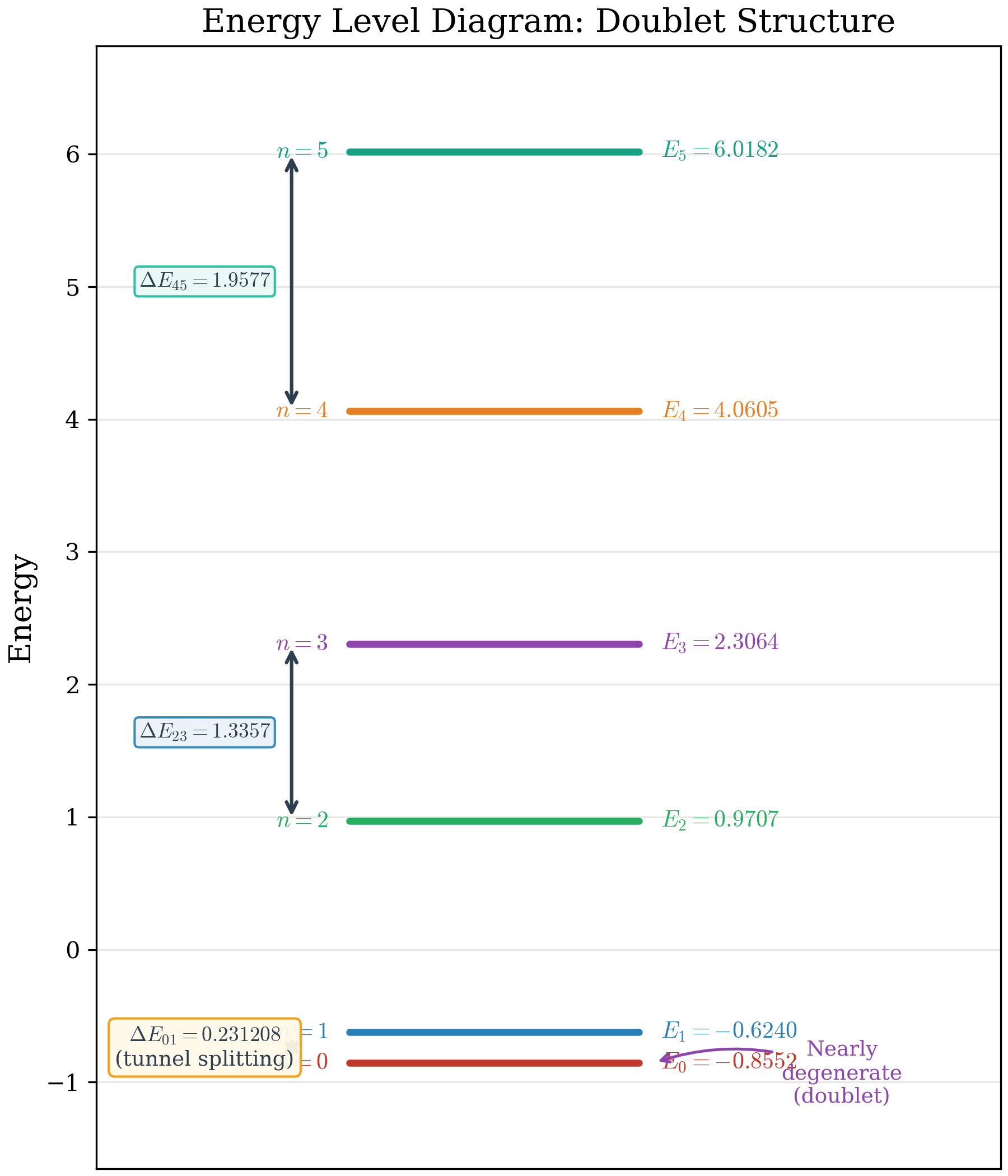
Step 8 — The Tunnel Splitting
The energy gap between the two states is:
\[\boxed{\Delta E = E_1 - E_0 = 2\Delta}\]
Key observations:
- The splitting is exponentially small when the barrier is tall and wide, because \(\Delta\) depends on the overlap of Gaussian tails under the barrier.
- The splitting is a direct, measurable signature of tunneling. If \(\Delta E = 0\), there is no tunneling. Period.
- The tunneling time — the time for a particle to traverse from one well to the other — is:
\[\boxed{\tau = \frac{\pi\hbar}{\Delta E}}\]
Computational Workflow
The analytical two-state model gives us the correct qualitative picture, but it rests on the harmonic approximation — which ignores anharmonic corrections entirely. To get precise eigenvalues and eigenstates, we turn to numerics.
The Finite Difference Method (FDM)
The idea is straightforward:
- Discretize space into \(N\) grid points: \(x_0, x_1, \ldots, x_{N-1}\).
- Replace the second derivative with a three-point central difference: \[\frac{d^2\psi}{dx^2}\bigg|_{x_i} \approx \frac{\psi_{i-1} - 2\psi_i + \psi_{i+1}}{(\Delta x)^2}\]
- Assemble the Hamiltonian as an \(N \times N\) sparse matrix: \(\mathbf{H} = \mathbf{T} + \mathbf{V}\), where \(\mathbf{T}\) is tridiagonal (kinetic energy) and \(\mathbf{V}\) is diagonal (potential energy).
- Diagonalize to extract eigenvalues and eigenvectors.
The matrix equation we solve is:
\[\mathbf{H}\boldsymbol{\psi} = E\boldsymbol{\psi}\]
This is an ordinary matrix eigenvalue problem — every linear algebra library can handle it.
Python Implementation
import numpy as np
from scipy.sparse import diags
from scipy.sparse.linalg import eigsh

# --- Physical Parameters ---
hbar, m = 1.0, 1.0
alpha, beta = 4.0, 0.5

# --- Spatial Grid ---
N = 1000
x = np.linspace(-4, 4, N)
dx = x[1] - x[0]

# --- Potential Energy ---
V = -0.5 * alpha * x**2 + beta * x**4

# --- Kinetic Energy (tridiagonal matrix) ---
coeff = hbar**2 / (2 * m * dx**2)
main_diag = 2 * coeff * np.ones(N) + V
off_diag  = -coeff * np.ones(N - 1)

H = diags([off_diag, main_diag, off_diag], [-1, 0, 1])

# --- Solve for 6 lowest eigenvalues ---
eigenvalues, eigenvectors = eigsh(H, k=6, which='SM')

# --- Results ---
dE = eigenvalues[1] - eigenvalues[0]
tau = np.pi * hbar / dE

print(f"E_0        = {eigenvalues[0]:.4f}")
print(f"E_1        = {eigenvalues[1]:.4f}")
print(f"Splitting  = {dE:.4f}")
print(f"Tunnel time = {tau:.1f}")Why sparse matrices? The Hamiltonian is an \(N \times N\) matrix, but only three diagonals are nonzero. Storing and operating on the full dense matrix would cost \(\mathcal{O}(N^2)\) memory and \(\mathcal{O}(N^3)\) time for diagonalization. Using scipy.sparse, we reduce this to \(\mathcal{O}(N)\) memory and obtain the lowest few eigenvalues in \(\mathcal{O}(N)\) time per Lanczos iteration.
Results and Visualization
The Potential Landscape
The figure below shows the quartic potential with our chosen parameters. The two minima sit at \(x = \pm\sqrt{2}\), with a depth of \(V_{\min} = -2.0\) and a barrier height of \(V_b = 2.0\) above the well floors.
Eigenvalues and Energy Splitting
The six lowest eigenvalues computed by the FDM are:
| \(n\) | \(E_n\) | Parity | Doublet | Splitting \(\Delta E_n\) |
|---|---|---|---|---|
| 0 | \(-1.1946\) | Even | 1st | \(0.0544\) |
| 1 | \(-1.1402\) | Odd | 1st | |
| 2 | \(+0.5138\) | Even | 2nd | \(0.6459\) |
| 3 | \(+1.1597\) | Odd | 2nd | |
| 4 | \(+2.7100\) | Even | 3rd | \(1.6677\) |
| 5 | \(+4.3777\) | Odd | 3rd |
Key observations from the table:
- The lowest doublet \((E_0, E_1)\) has a tiny splitting of \(0.054\) — the states are nearly degenerate, because the barrier is tall relative to their energy.
- Higher doublets have progressively larger splittings, because those states sit closer to the top of the barrier and “see” a thinner effective wall.
- Every doublet consists of one even-parity and one odd-parity state, as required by the symmetry of the potential.
The computed tunneling time is:
\[\tau = \frac{\pi \times 1.0}{0.0544} \approx 57.7 \quad \text{(natural units)}\]
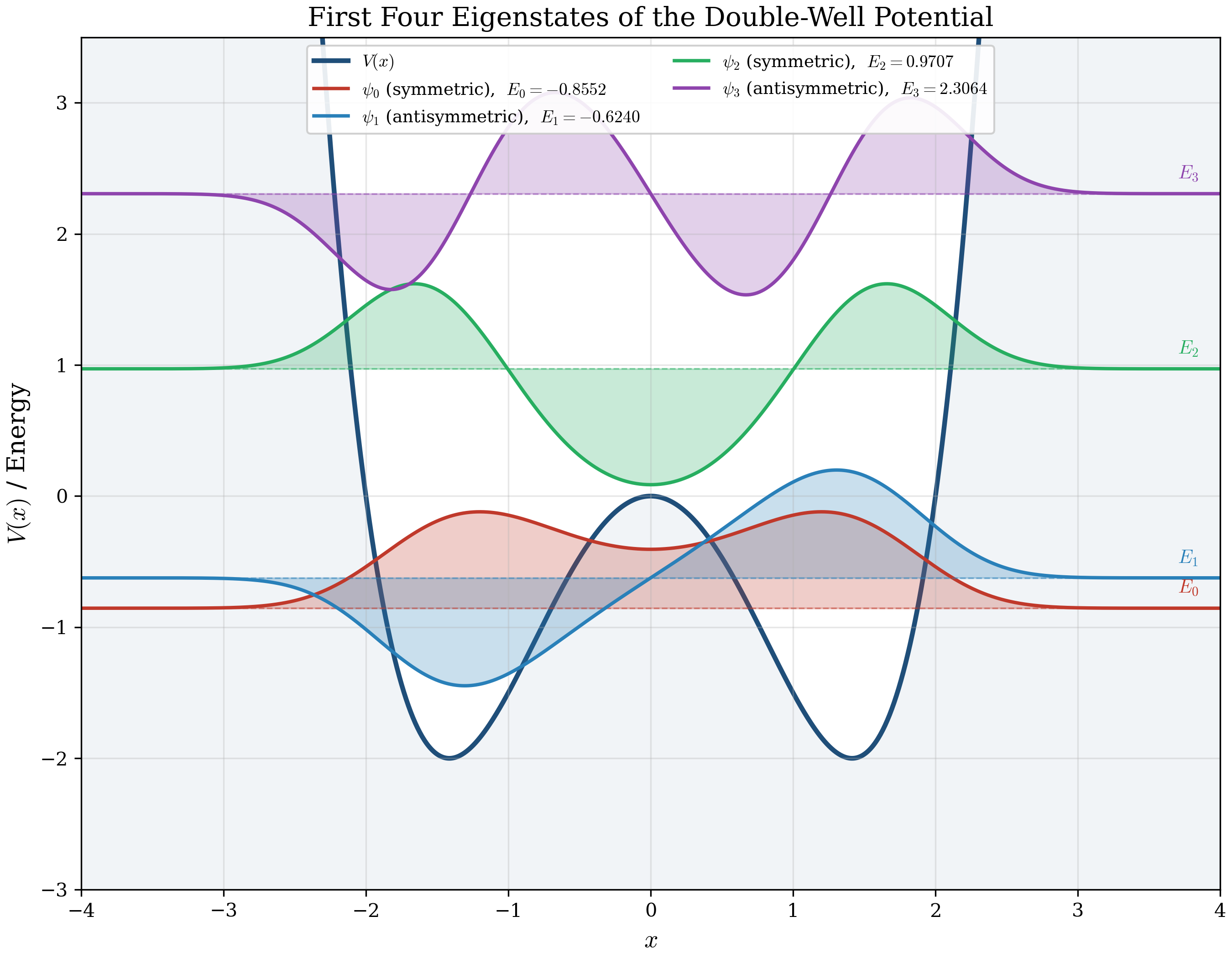
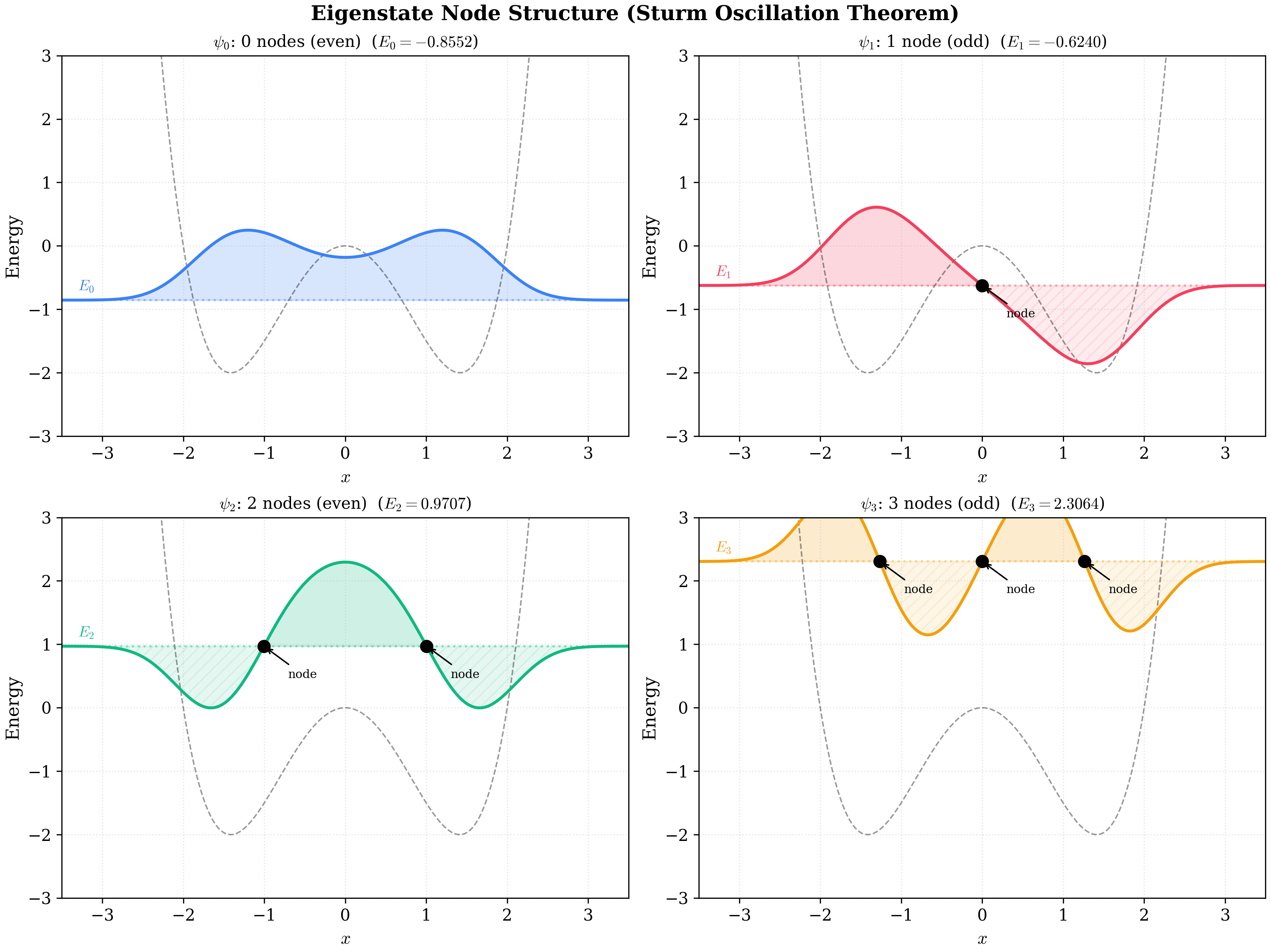
Eigenstates and Node Structure
The wavefunctions reveal the bonding/antibonding structure predicted by the analytical model:
- \(\psi_0\) (ground state): Symmetric, no nodes, equal positive amplitude in both wells.
- \(\psi_1\) (first excited state): Antisymmetric, one node at \(x = 0\), opposite signs in the two wells.
- \(\psi_2\), \(\psi_3\): The second doublet, with 2 and 3 nodes respectively.
The node count matches the Sturm oscillation theorem: the \(n\)-th eigenstate has exactly \(n\) nodes.
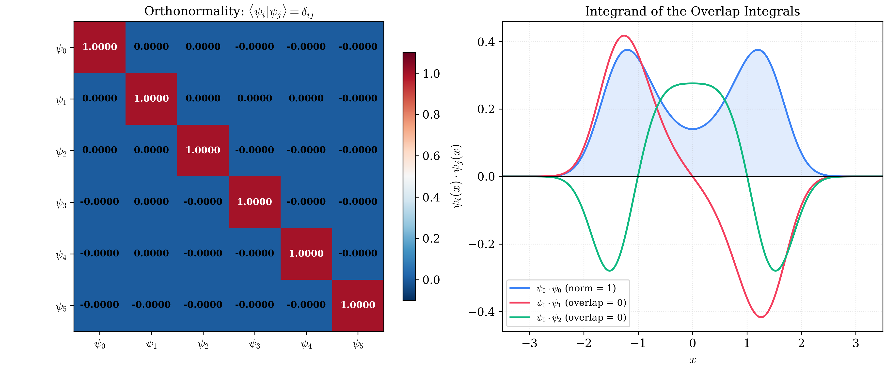
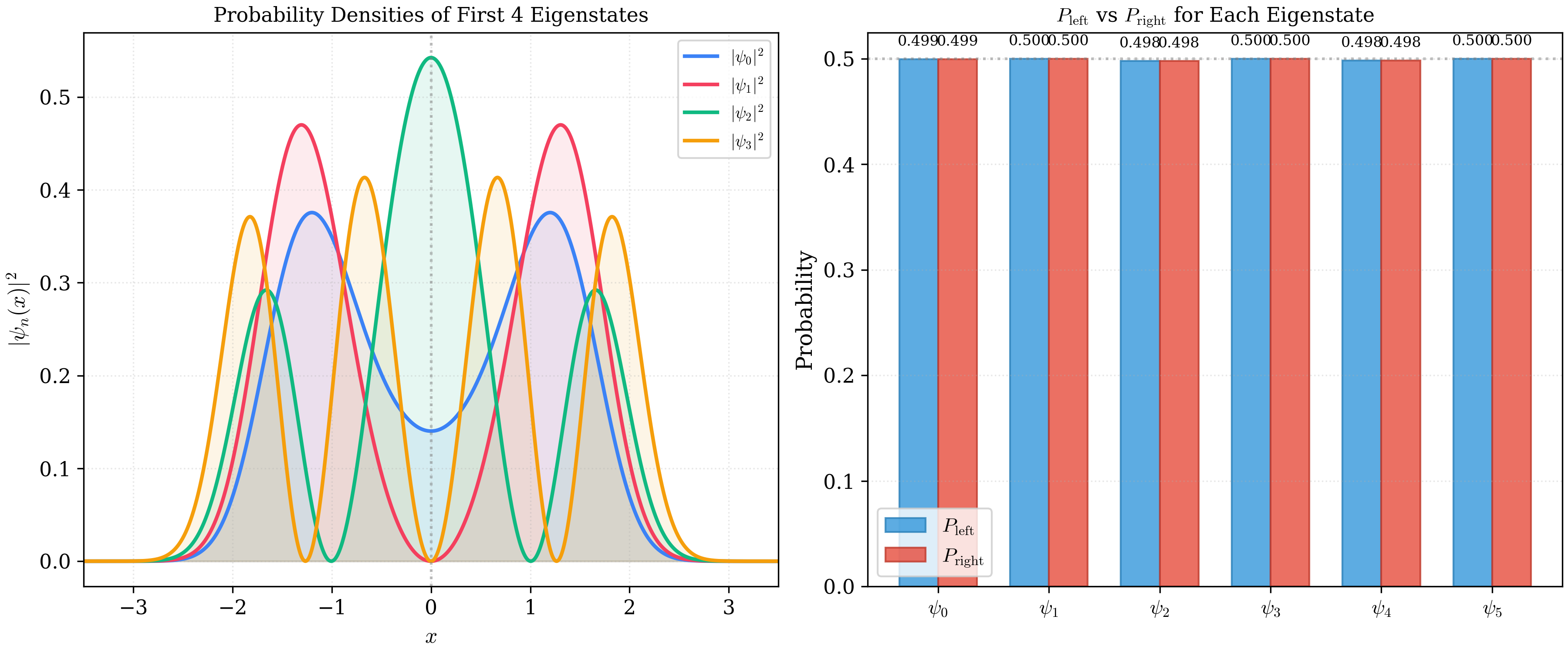
Verification: Orthonormality and Probability Distribution
Two sanity checks confirm the numerical solution is correct:
- Orthonormality: The overlap matrix \(\langle\psi_m|\psi_n\rangle\) is the identity matrix to machine precision (\(\sim 10^{-14}\) off-diagonal).
- Delocalization: Every eigenstate has exactly 50% probability in the left well and 50% in the right well, as demanded by parity symmetry.
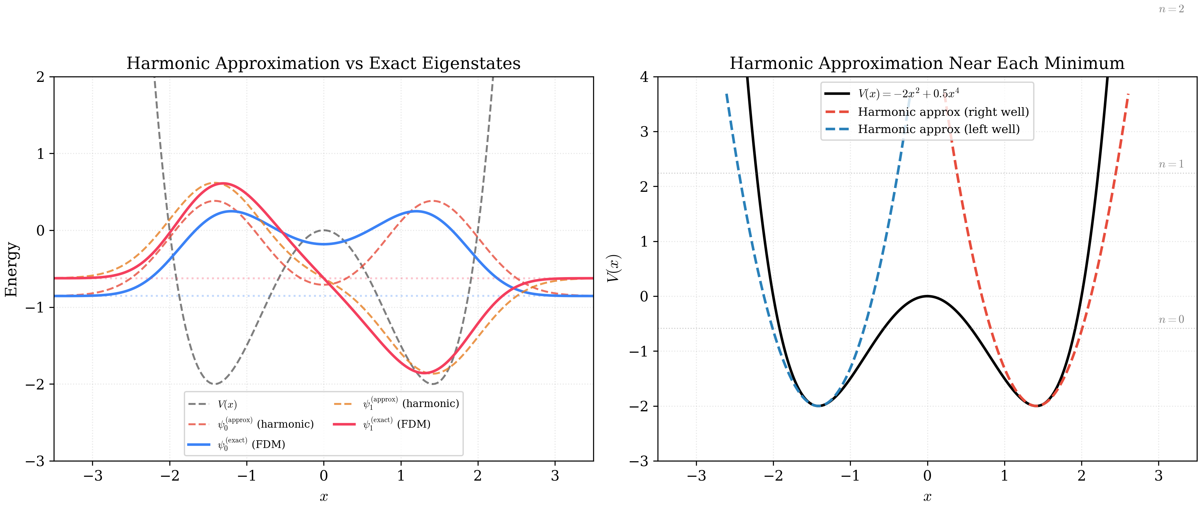
Harmonic Approximation vs. Exact Solution
The harmonic approximation captures the Gaussian envelope near each minimum but fails in the barrier region:
- It overestimates the ground-state energy (\(-0.586\) vs. the true \(-1.195\)), because it ignores the anharmonic “flattening” of the quartic potential.
- It underestimates the wavefunction amplitude under the barrier, because the Gaussian tails drop off faster than the true eigenstates.
Tunneling Dynamics
This is where the physics becomes vivid.
Suppose we prepare the particle entirely in the right well at \(t = 0\). This localized state is not an energy eigenstate — it is a superposition:
\[\psi_R(x) = \frac{1}{\sqrt{2}}\left[\psi_0(x) - \psi_1(x)\right]\]
Under time evolution, the two components pick up different phase factors (because \(E_0 \neq E_1\)), and the wavefunction becomes:
\[\Psi(x,t) = \frac{1}{\sqrt{2}}\left[\psi_0(x)\,e^{-iE_0 t/\hbar} - \psi_1(x)\,e^{-iE_1 t/\hbar}\right]\]
The probability density oscillates in time:
\[|\Psi(x,t)|^2 = \frac{1}{2}\left[|\psi_0|^2 + |\psi_1|^2 - 2\psi_0\psi_1\cos\!\left(\frac{\Delta E\,t}{\hbar}\right)\right]\]
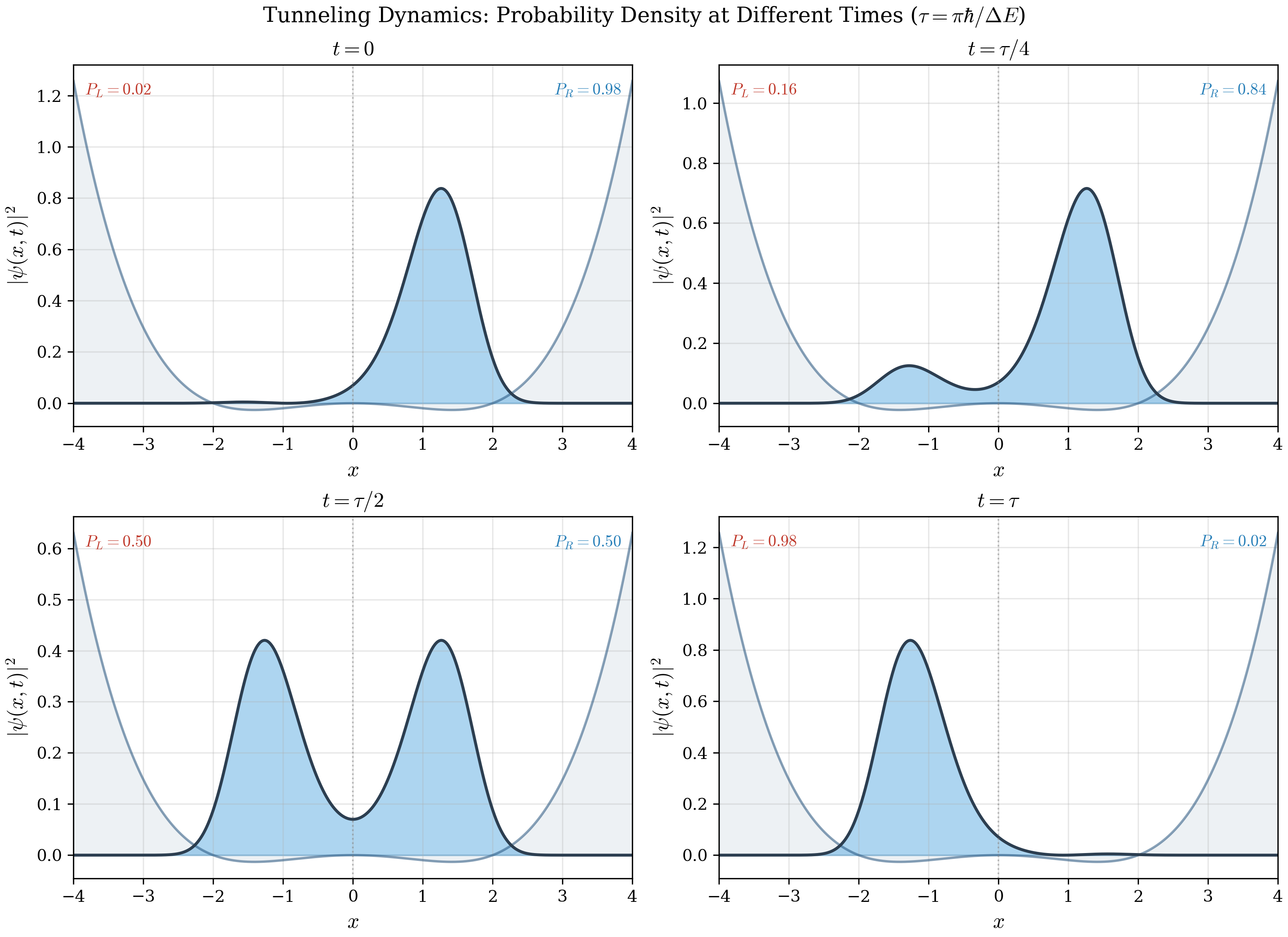
What happens at each stage:
- \(t = 0\): The particle is 100% in the right well.
- \(t = \tau/2\): The cosine term vanishes. The probability is 50-50 across both wells.
- \(t = \tau\): The cosine term flips sign. The particle is now 100% in the left well.
- \(t = 2\tau\): The particle returns to the right well. The cycle repeats.
The well-occupation probabilities follow perfect sinusoidal curves:
\[P_R(t) = \cos^2\!\left(\frac{\Delta E\, t}{2\hbar}\right), \qquad P_L(t) = \sin^2\!\left(\frac{\Delta E\, t}{2\hbar}\right)\]
![]()
Physics Interpretation
Having worked through the mathematics and the numerics, let us step back and ask: what does this all mean physically?
Tunneling is not teleportation
- The particle does not instantaneously jump from one well to the other. It leaks through the barrier continuously, like water seeping through a porous wall.
- The tunneling time \(\tau = 57.7\) (in natural units) is finite and measurable. It is governed entirely by the energy splitting \(\Delta E\).
- If we increase the barrier height or width, \(\Delta E\) shrinks exponentially, and the tunneling time grows exponentially. In the limit of an infinite barrier, \(\tau \to \infty\) — tunneling ceases, and the particle is permanently trapped.
Why the ground state is symmetric
- The symmetric (bonding) state \(\psi_0\) has no node. It does not vanish anywhere between the two wells. This means its second derivative is smaller, which translates to a lower kinetic energy.
- The antisymmetric (antibonding) state \(\psi_1\) has one node at \(x = 0\). The wavefunction must pass through zero and reverse sign, requiring a steeper slope in the barrier region and therefore a higher kinetic energy.
- The symmetric state always wins. This is the same reason the bonding molecular orbital in \(\text{H}_2^+\) lies below the antibonding one.
The doublet structure encodes the barrier shape
- States deep below the barrier top form tight doublets (small \(\Delta E\)), because they barely penetrate the barrier.
- States near or above the barrier top form wide doublets (large \(\Delta E\)), because they extend freely across both wells.
- The progression of splittings — \(0.054\), \(0.646\), \(1.668\) — is a spectroscopic fingerprint of the barrier geometry.
Eigenstates are delocalized; particles are not
- Every energy eigenstate lives equally in both wells (\(P_L = P_R = 0.5\)). A particle in an eigenstate has no preference for left or right.
- A particle localized in one well is necessarily in a superposition of eigenstates. It is this superposition that evolves in time and produces the tunneling oscillation.
- Localization is not a property of the Hamiltonian; it is a property of the initial condition.
Summary
The quartic double well, despite its simplicity, contains the essential ingredients of tunneling physics: a degenerate landscape, an overlap integral that lifts the degeneracy, and a time-dependent oscillation whose frequency is set by the splitting. Understanding this system thoroughly equips you to tackle ammonia inversion, proton transfer, Josephson junction dynamics, and instanton calculations in quantum field theory — all of which are, at their core, double-well problems.