In physics and engineering, exact analytical solutions are often impossible to obtain for complex, real-world systems. Whether simulating fluid dynamics around an airfoil, calculating the chaotic orbits of celestial bodies, or modeling the wavefunction of a multi-electron atom, computational scientists rely on numerical approximations.
However, approximations inherently introduce errors. Understanding the sources, behavior, and propagation of these errors is the cornerstone of numerical analysis. Without a rigorous grasp of error bounds, a simulation of a bridge’s structural integrity might yield catastrophically incorrect results without the engineer realizing it. This module introduces the fundamental types of errors encountered in numerical computing and provides the mathematical tools to quantify and mitigate them.
2. Theory: Types of Errors and Error Metrics
2.1 Error Definitions
When an approximate value \(p^*\) is used to represent a true (exact) value \(p\), we define the following metrics to quantify the discrepancy:
True Error (\(E_t\)): The exact difference between the true value and the approximation. \[ E_t = p - p^* \]
Absolute Error (\(|E_t|\)): The magnitude of the error. \[ |E_t| = |p - p^*| \]
Relative Error (\(E_r\)): The error scaled by the true value, often expressed as a percentage. This is typically more useful than absolute error because it normalizes the error magnitude relative to the scale of the value being measured. \[ E_r = \frac{p - p^*}{p} \]\[ \text{Percent Relative Error } (\varepsilon_t) = \left| \frac{p - p^*}{p} \right| \times 100\% \]
In most numerical algorithms, the true value \(p\) is unknown (which is why we are approximating it in the first place!). In iterative methods, we instead calculate the Approximate Relative Error (\(\varepsilon_a\)): \[ \varepsilon_a = \left| \frac{\text{Current Approximation} - \text{Previous Approximation}}{\text{Current Approximation}} \right| \times 100\% \]
2.2 Significant Figures
Significant figures (or digits) relate to the confidence we have in an approximation. A number \(p^*\) is said to approximate \(p\) to \(t\) significant digits if \(t\) is the largest non-negative integer for which: \[ \frac{|p - p^*|}{|p|} \le 5 \times 10^{-t} \]
2.3 Sources of Error
There are two primary sources of numerical errors:
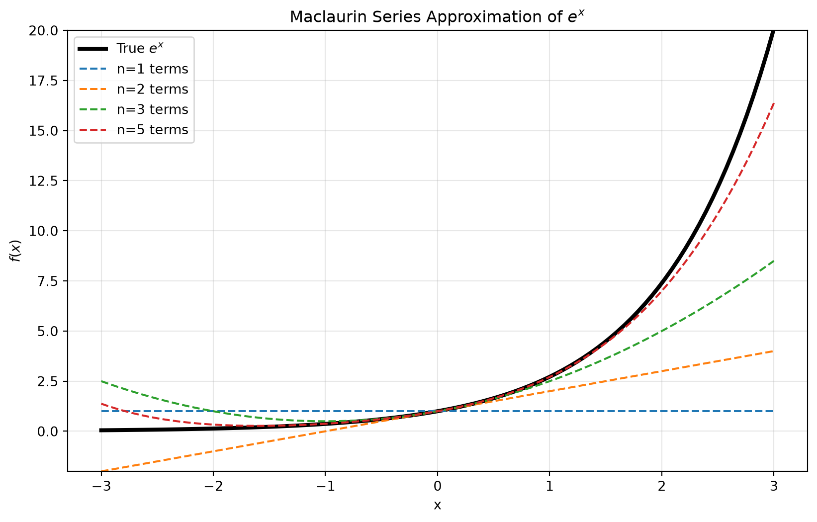
Truncation Error: Arises when mathematical procedures are formulated using an infinite number of operations, but are truncated to a finite number of steps for computation. A classic example is the truncation of a Taylor series.
The Taylor series expansion of a sufficiently smooth function \(f(x)\) about a point \(x = a\) is: \[ f(x) = f(a) + f'(a)(x-a) + \frac{f''(a)}{2!}(x-a)^2 + \dots + \frac{f^{(n)}(a)}{n!}(x-a)^n + R_n(x) \] where \(R_n(x)\) is the Remainder (or truncation error), given by: \[ R_n(x) = \frac{f^{(n+1)}(\xi)}{(n+1)!}(x-a)^{n+1} \] for some \(\xi\) between \(a\) and \(x\).
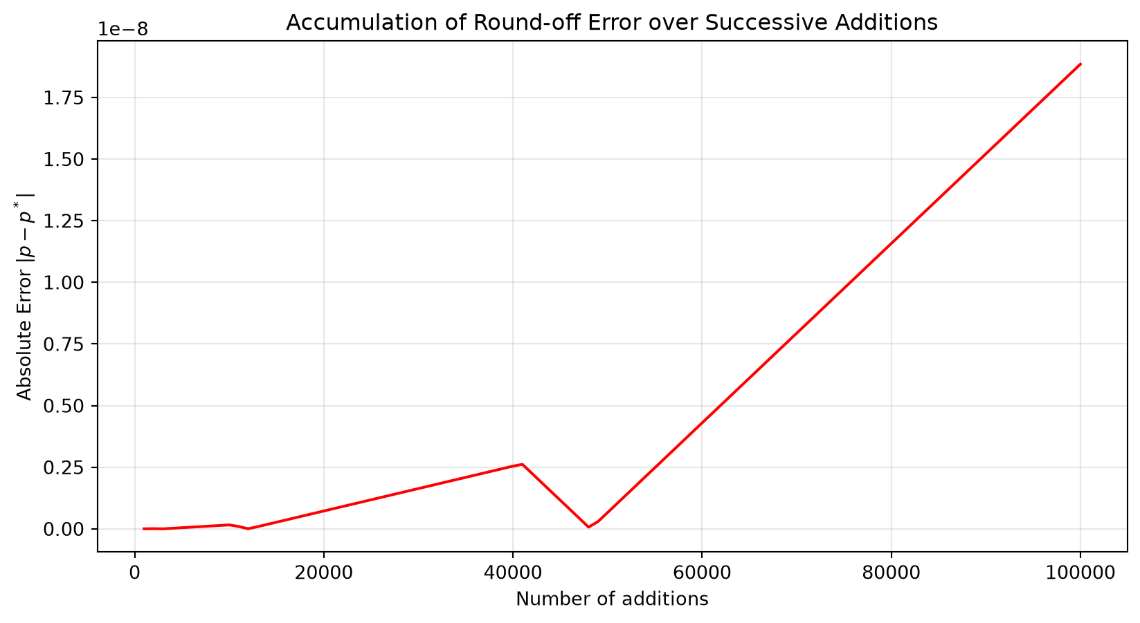
Round-off Error: Arises because computers represent real numbers using a finite number of bits (floating-point representation). This introduces a minimum resolvable difference between distinct numbers, known as Machine Epsilon (\(\epsilon_{mach}\)). In double-precision IEEE 754 floating-point format, \(\epsilon_{mach} \approx 2.22 \times 10^{-16}\).
A severe consequence of round-off error is Subtractive (or Catastrophic) Cancellation. This occurs when subtracting two nearly equal numbers, leading to a massive loss of significant digits.
2.4 Error Propagation
When operations are performed on approximate numbers, errors propagate. For an arithmetic operation involving variables \(x\) and \(y\) with absolute errors \(\Delta x\) and \(\Delta y\):
Addition/Subtraction (\(z = x \pm y\)): Absolute errors add up. \(\Delta z \approx \Delta x + \Delta y\)
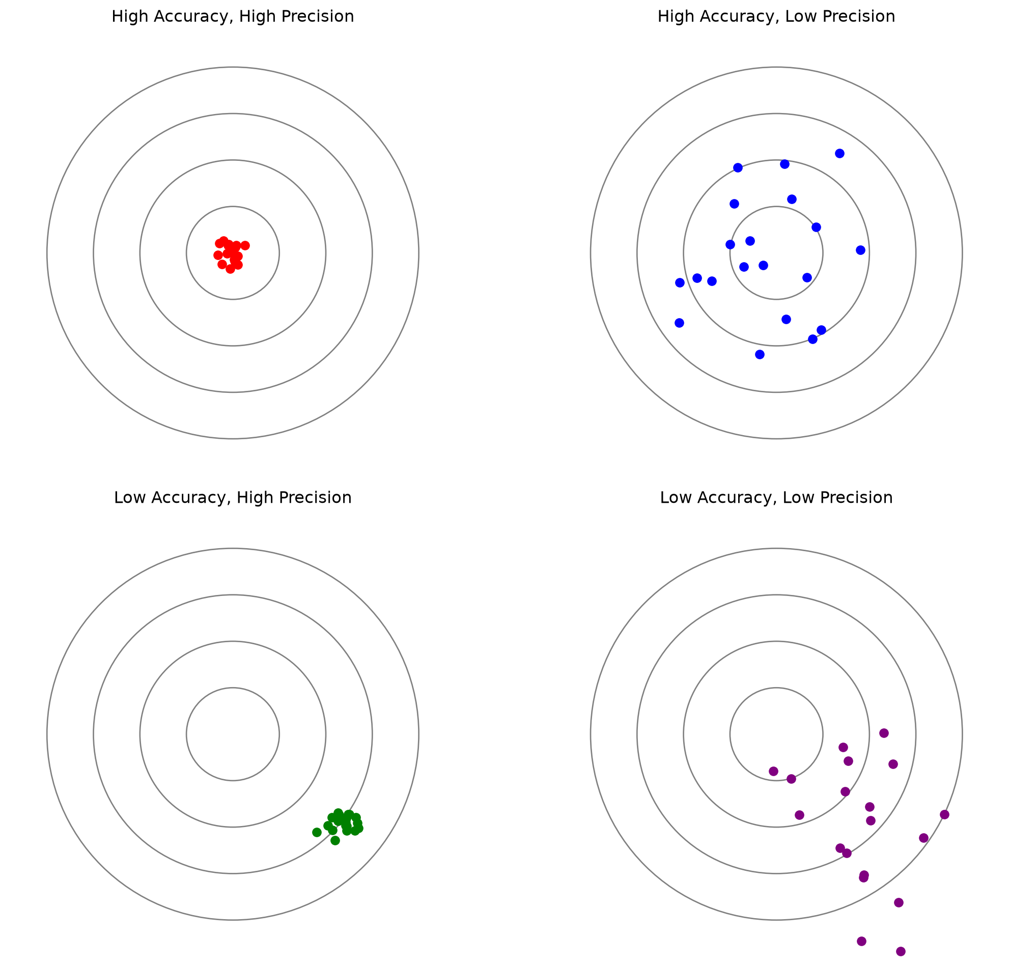
Accuracy: How closely a computed or measured value agrees with the true value. (Characterized by low bias).
Precision: How closely individual computed or measured values agree with each other. (Characterized by low variance or standard deviation).
3. Geometric/Visual Explanation
Let’s visualize the concepts of truncation error, accuracy vs. precision, and error propagation using Python.
3.1 Truncation Error in Taylor Series
import numpy as npimport matplotlib.pyplot as pltimport mathx_vals = np.linspace(-3, 3, 100)y_true = np.exp(x_vals)plt.figure(figsize=(10, 6))plt.plot(x_vals, y_true, 'k-', linewidth=3, label="True $e^x$")# Calculate Taylor approximationsfor n in [1, 2, 3, 5]: y_approx = np.zeros_like(x_vals)for i inrange(n): y_approx += (x_vals**i) / math.factorial(i) plt.plot(x_vals, y_approx, '--', label=f"n={n} terms")plt.title("Maclaurin Series Approximation of $e^x$")plt.xlabel("x")plt.ylabel("$f(x)$")plt.ylim(-2, 20)plt.grid(True, alpha=0.3)plt.legend()plt.show()
Figure 1: Convergence of Maclaurin series for \(e^x\) as the number of terms increases. The truncation error decreases as more terms are added.
3.2 Accuracy vs Precision (Dartboard Analogy)
plt.figure(figsize=(12, 10))def draw_dartboard(ax, title): circles = [plt.Circle((0,0), r, fill=False, color='gray') for r in [0.25, 0.5, 0.75, 1.0]]for c in circles: ax.add_artist(c) ax.set_xlim(-1.2, 1.2) ax.set_ylim(-1.2, 1.2) ax.set_aspect('equal') ax.set_title(title) ax.axis('off')# Accurate and Preciseax1 = plt.subplot(221)draw_dartboard(ax1, "High Accuracy, High Precision")ax1.scatter(np.random.normal(0, 0.05, 20), np.random.normal(0, 0.05, 20), color='red')# Accurate but Impreciseax2 = plt.subplot(222)draw_dartboard(ax2, "High Accuracy, Low Precision")ax2.scatter(np.random.normal(0, 0.3, 20), np.random.normal(0, 0.3, 20), color='blue')# Inaccurate but Preciseax3 = plt.subplot(223)draw_dartboard(ax3, "Low Accuracy, High Precision")ax3.scatter(np.random.normal(0.6, 0.05, 20), np.random.normal(-0.5, 0.05, 20), color='green')# Inaccurate and Impreciseax4 = plt.subplot(224)draw_dartboard(ax4, "Low Accuracy, Low Precision")ax4.scatter(np.random.normal(0.5, 0.3, 20), np.random.normal(-0.5, 0.3, 20), color='purple')plt.tight_layout()plt.show()
Figure 2: Scatter plots illustrating the difference between Accuracy (proximity to the center/truth) and Precision (tightness of the cluster).
3.3 Error Propagation (Round-off Accumulation)
N =100000true_value =0.1* Napprox_sum =0.0errors = []for i inrange(1, N +1): approx_sum +=0.1if i %1000==0: errors.append(abs(approx_sum - (i *0.1)))plt.figure(figsize=(10, 5))plt.plot(range(1000, N +1, 1000), errors, 'r-')plt.title("Accumulation of Round-off Error over Successive Additions")plt.xlabel("Number of additions")plt.ylabel("Absolute Error $|p - p^*|$")plt.grid(True, alpha=0.3)plt.ticklabel_format(axis='y', style='sci', scilimits=(0,0))plt.show()
Figure 3: Accumulation of round-off error when successively adding \(0.1\) to a sum \(100{,}000\) times.
4. Python Implementation
The following Python code demonstrates how to iteratively compute a Taylor series until a desired approximate relative error tolerance is met.
def exp_maclaurin(x, es=0.0001, max_iter=50):""" Approximates e^x using the Maclaurin series. Parameters: x (float): The exponent. es (float): Stopping criterion (percent relative error tolerance). max_iter (int): Maximum number of iterations. Returns: tuple: (approximation, iterations, approximate_relative_error_history) """ approx =1.0# First term (n=0) term =1.0 ea_history = []for n inrange(1, max_iter +1): prev_approx = approx term = term * x / n approx += termif approx !=0: ea =abs((approx - prev_approx) / approx) *100else: ea =float('inf') ea_history.append(ea)if ea < es:return approx, n, ea_historyprint(f"Warning: Maximum iterations ({max_iter}) reached.")return approx, max_iter, ea_history# Example usageval, iters, eas = exp_maclaurin(1.5, es=0.05)print(f"Approximation of e^1.5: {val}")print(f"True value of e^1.5: {math.exp(1.5)}")print(f"Iterations required: {iters}")
Approximation of e^1.5: 4.48156476702009
True value of e^1.5: 4.4816890703380645
Iterations required: 8
5. Solved Examples
🟢 Easy Example: Basic Error Metrics
Problem: A student measures the length of a bridge to be \(99.99 \, \text{m}\) and a rivet to be \(9 \, \text{cm} = 0.09 \, \text{m}\). The true length of the bridge is \(100.00 \, \text{m}\) and the true length of the rivet is \(10 \, \text{cm} = 0.10 \, \text{m}\). Calculate the true error and percent relative error for each measurement.
Insight: Although the absolute error is exactly the same (\(0.01 \, \text{m}\)) for both, the relative error shows that the bridge measurement is vastly superior.
🟡 Medium Example: Iterative Errors
Problem: Approximate \(e^{0.5}\) using Maclaurin series terms up to \(n=3\). Compute the true value, absolute error, and percent approximate relative error at each step.
Solution:
True value: \(e^{0.5} \approx 1.648721\)
Term (n)
Addition
Approximation (\(p^*\))
\(\|E_t\| = \|p - p^*\|\)
\(\varepsilon_a\) (%)
\(n=0\)
\(1\)
\(1.0\)
\(0.648721\)
-
\(n=1\)
\(0.5\)
\(1.5\)
\(0.148721\)
\(33.3\%\)
\(n=2\)
\(0.125\)
\(1.625\)
\(0.023721\)
\(7.69\%\)
\(n=3\)
\(0.02083\)
\(1.645833\)
\(0.002888\)
\(1.27\%\)
As terms increase, true error decreases, and the approximate relative error serves as a useful gauge for this convergence.
🔴 Hard Example: Catastrophic Cancellation in the Quadratic Formula
Problem: Consider the quadratic equation \(x^2 - 100000.00001x + 1 = 0\). Use the standard quadratic formula to find the roots, and demonstrate subtractive cancellation for the smaller root. Show how to mathematically reformulate the calculation to avoid this error.
Solution:
The roots are given by \(x = \frac{-b \pm \sqrt{b^2 - 4ac}}{2a}\). Here, \(a = 1\), \(b = -100000.00001\), \(c = 1\).
a =1.0b =-100000.00001c =1.0# Standard Formuladiscriminant = math.sqrt(b**2-4*a*c)x1_std = (-b + discriminant) / (2*a)x2_std = (-b - discriminant) / (2*a) # Subtractive cancellation occurs here!print(f"Standard Formula x1: {x1_std}")print(f"Standard Formula x2 (loss of precision): {x2_std}")# Reformulated Formula to avoid cancellation for the smaller rootx2_alt = (2* c) / (-b + discriminant)print(f"Reformulated Formula x2 (accurate): {x2_alt}")print(f"Check x1 * x2 = c/a: {x1_std * x2_alt == c/a}")
Standard Formula x1: 100000.0
Standard Formula x2 (loss of precision): 1.0000003385357559e-05
Reformulated Formula x2 (accurate): 1e-05
Check x1 * x2 = c/a: True
Insight: In calculating \(x_2\) with the standard formula, we subtracted two nearly identical large numbers (\(-b\) and \(\sqrt{b^2-4ac}\)). This stripped away significant digits. By rationalizing the numerator, we converted the problematic subtraction into an addition, completely mitigating the catastrophic cancellation.
6. Practice Problems
Find the true error, absolute error, and percent relative error when \(p = \pi\) is approximated by \(p^* = 22/7\).
Determine the number of significant digits to which \(p^* = 0.54032\) approximates \(p = \cos(1)\).
Use the zero-order, first-order, and second-order Taylor series expansions to predict \(f(3)\) for \(f(x) = 25x^3 - 6x^2 + 7x - 88\) using a base point at \(x=1\). Calculate the true relative error for each approximation.
Calculate the machine epsilon \(\epsilon_{mach}\) for your computer system by writing a small Python script that iteratively halves a value \(e = 1.0\) until \(1.0 + e == 1.0\).
Consider calculating \(f(x) = \frac{1 - \cos(x)}{x^2}\) for very small \(x\) (e.g., \(x = 10^{-6}\)). Explain why computing this directly leads to high errors, and use a Taylor expansion of \(\cos(x)\) to derive a stable formula.
7. Summary
Key Takeaways and Formulas
Numerical approximations introduce errors that must be managed to ensure valid computational results.
Truncation Error arises from using a finite number of steps for a mathematically infinite procedure (e.g., dropping higher-order terms in a Taylor series).
Round-off Error is caused by the finite precision of computer memory (floating-point representation).
Catastrophic Cancellation occurs when subtracting two nearly equal numbers, leading to a severe loss of significant digits. It can often be fixed by algebraic rearrangement.