Module 2: Computer Programming for Numerical Methods

Author Physics Course Writer

Published October 1, 2026

Copied!

1 Introduction

In numerical analysis, the transition from analytical mathematical derivations to practical computation requires a robust programming environment. Numerical methods are algorithmic by nature; they involve repeated calculations, iterative updates, and handling large arrays of data. This module bridges the gap between pure mathematics and computational execution, focusing on the fundamental programming concepts necessary for implementing numerical methods.

In modern physics and engineering, Python has become the lingua franca for scientific computing. Its syntax is intuitive and closely mimics mathematical notation, while its vast ecosystem of libraries—specifically NumPy, SciPy, and Matplotlib—provides powerful tools for array operations, linear algebra, and data visualization.

This module will cover why Python is chosen for numerical computing, how to leverage NumPy for high-performance vectorized operations, how to visualize results using Matplotlib, and how to structure code into reusable, modular functions with robust convergence checks.

2 Theory and Concepts

2.1 Why Python for Numerical Computing?

Python is an interpreted, high-level language. While standard Python lists and loops can be slow compared to compiled languages like C or Fortran, libraries like NumPy wrap highly optimized C and Fortran code. This allows us to write code quickly in Python while achieving performance comparable to low-level languages, provided we use vectorization.

2.2 NumPy Arrays and Vectorization

A NumPy array (ndarray) is a grid of values, all of the same type. Vectorization is the process of performing mathematical operations on these arrays without explicit for loops in Python.

For example, given vectors \(\mathbf{u}\) and \(\mathbf{v}\), computing \(\mathbf{w} = \mathbf{u} + \mathbf{v}\) element-wise is written simply as w = u + v in NumPy.

2.3 Loops, Conditionals, and Convergence Checks

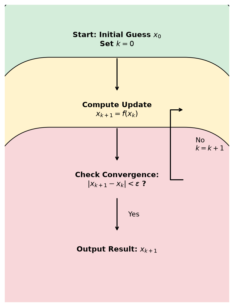
Iterative numerical methods (like finding roots or solving differential equations) rely on loops. A while loop is typically used when the number of iterations is unknown, but a tolerance condition must be met.

The convergence check usually looks like: \[|x_{k+1} - x_k| < \epsilon\] where \(\epsilon\) is the specified tolerance. To prevent infinite loops (e.g., if the method diverges), we must always include a maximum iteration counter max_iter.

2.4 Best Practices

1. Commenting and Docstrings: Explain why code does what it does. Document function inputs, outputs, and side effects.
2. Modular Code: Break complex algorithms into smaller, testable functions.
3. Avoid Magic Numbers: Define physical constants and algorithm parameters (like tolerance) as variables.

3 Geometric and Visual Explanations

In this section, we utilize Python to illustrate core concepts visually.

3.1 1. Loop vs Vectorized Computation Speed

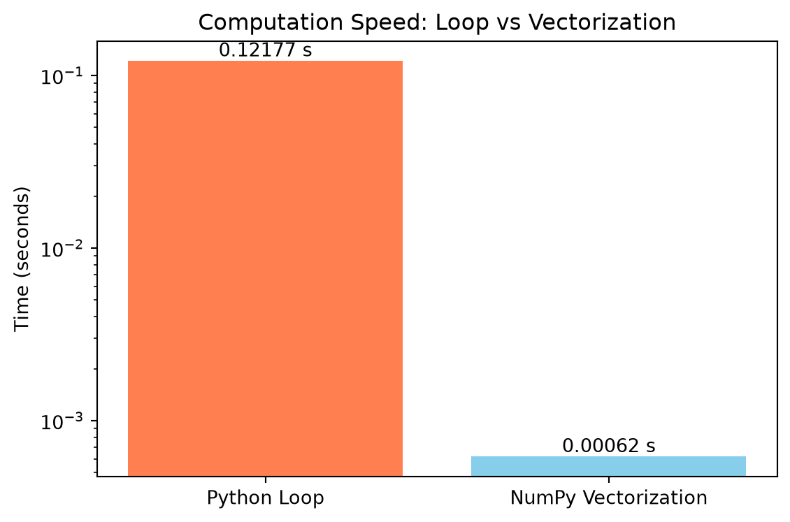
Vectorized operations in NumPy are drastically faster than standard Python loops. Let’s visualize this difference.

import numpy as np
import time
import matplotlib.pyplot as plt

# Size of the array
N = 1000000
x = np.random.rand(N)
y = np.random.rand(N)

# Method 1: Python Loop
start_time = time.time()
z_loop = np.zeros(N)
for i in range(N):
    z_loop[i] = x[i] * y[i]
loop_time = time.time() - start_time

# Method 2: Vectorization
start_time = time.time()
z_vec = x * y
vec_time = time.time() - start_time

methods = ['Python Loop', 'NumPy Vectorization']
times = [loop_time, vec_time]

plt.figure(figsize=(6, 4))
bars = plt.bar(methods, times, color=['coral', 'skyblue'])
plt.ylabel('Time (seconds)')
plt.title('Computation Speed: Loop vs Vectorization')
plt.yscale('log') # Log scale for better visibility

# Add text annotations
for bar in bars:
    yval = bar.get_height()
    plt.text(bar.get_x() + bar.get_width()/2, yval, f"{yval:.5f} s", 
             ha='center', va='bottom')

plt.tight_layout()
plt.show()

Figure 1: Comparison of computation time between Python loops and NumPy vectorization.

3.2 2. Matplotlib Showcase

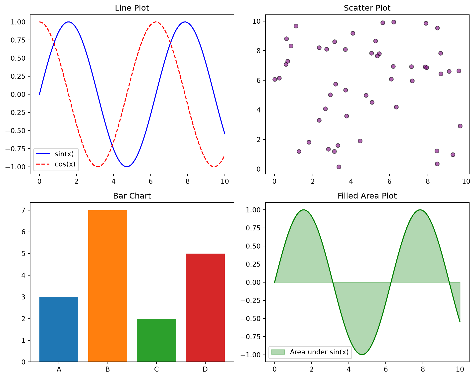
Visualizing data is critical in numerical analysis. Here is a showcase of common plots using a 2x2 subplot grid.

fig, axs = plt.subplots(2, 2, figsize=(10, 8))

# Data
x = np.linspace(0, 10, 100)
y1 = np.sin(x)
y2 = np.cos(x)
x_scatter = np.random.rand(50) * 10
y_scatter = np.random.rand(50) * 10
categories = ['A', 'B', 'C', 'D']
values = [3, 7, 2, 5]

# Top-Left: Line Plot
axs[0, 0].plot(x, y1, label='sin(x)', color='blue')
axs[0, 0].plot(x, y2, label='cos(x)', color='red', linestyle='--')
axs[0, 0].set_title('Line Plot')
axs[0, 0].legend()

# Top-Right: Scatter Plot
axs[0, 1].scatter(x_scatter, y_scatter, color='purple', alpha=0.6, edgecolors='k')
axs[0, 1].set_title('Scatter Plot')

# Bottom-Left: Bar Chart
axs[1, 0].bar(categories, values, color=['#1f77b4', '#ff7f0e', '#2ca02c', '#d62728'])
axs[1, 0].set_title('Bar Chart')

# Bottom-Right: Filled Area
axs[1, 1].fill_between(x, y1, alpha=0.3, color='green', label='Area under sin(x)')
axs[1, 1].plot(x, y1, color='green')
axs[1, 1].set_title('Filled Area Plot')
axs[1, 1].legend()

plt.tight_layout()
plt.show()

Figure 2: A 2x2 grid showcasing different Matplotlib plotting styles.

3.3 3. Iterative Method Flowchart

Most numerical methods follow a generic iterative structure. The following diagram illustrates this workflow.

import matplotlib.patches as patches

fig, ax = plt.subplots(figsize=(6, 8))
ax.axis('off')

def draw_box(ax, text, xy, width, height, boxstyle="round,pad=0.3", color="lightblue"):
    box = patches.FancyBboxPatch(xy, width, height, boxstyle=boxstyle, 
                                 edgecolor="black", facecolor=color)
    ax.add_patch(box)
    ax.text(xy[0] + width/2, xy[1] + height/2, text, ha='center', va='center', fontsize=11, fontweight='bold')

def draw_arrow(ax, xy_from, xy_to):
    ax.annotate("", xy=xy_to, xytext=xy_from,
                arrowprops=dict(arrowstyle="->", lw=1.5))

# Draw blocks
draw_box(ax, "Start: Initial Guess $x_0$\nSet $k = 0$", (0.2, 0.8), 0.6, 0.1, color="#cce5ff")
draw_box(ax, "Compute Update\n$x_{k+1} = f(x_k)$", (0.2, 0.6), 0.6, 0.1, color="#d4edda")
draw_box(ax, "Check Convergence:\n$|x_{k+1} - x_k| < \\epsilon$ ?", (0.2, 0.4), 0.6, 0.1, color="#fff3cd")
draw_box(ax, "Output Result: $x_{k+1}$", (0.2, 0.2), 0.6, 0.1, color="#f8d7da")

# Draw Main Arrows
draw_arrow(ax, (0.5, 0.8), (0.5, 0.7))
draw_arrow(ax, (0.5, 0.6), (0.5, 0.5))
draw_arrow(ax, (0.5, 0.4), (0.5, 0.3))

# Draw Loop Arrow (No convergence)
ax.annotate("", xy=(0.8, 0.65), xytext=(0.8, 0.45),
            arrowprops=dict(arrowstyle="->", lw=1.5, connectionstyle="bar,fraction=-0.2"))
ax.text(0.85, 0.55, "No\n$k = k+1$", ha='left', va='center', fontsize=10)

# Label Yes
ax.text(0.55, 0.35, "Yes", ha='left', va='center', fontsize=10)

plt.xlim(0, 1)
plt.ylim(0.1, 0.95)
plt.show()

Figure 3: Flowchart of a generic iterative numerical method.

4 Python Implementation

In this section, we showcase properly structured numerical code, adhering to the best practices described earlier.

5 Solved Examples

5.1 🟢 Easy: Factorial and Taylor Series

Problem: Write a function to compute the factorial of a number. Use it to compute the first 5 terms of the Taylor series approximation for \(e^x\) at \(x = 1\). The Taylor series is \(e^x \approx \sum_{n=0}^{\infty} \frac{x^n}{n!}\).

Solution:

def compute_factorial(n):
    """Computes the factorial of n (n!)."""
    if n == 0 or n == 1:
        return 1
    result = 1
    for i in range(2, n + 1):
        result *= i
    return result

def approx_exp(x, terms):
    """Approximates e^x using Taylor series up to 'terms' terms."""
    approx = 0.0
    for n in range(terms):
        approx += (x**n) / compute_factorial(n)
    return approx

x_val = 1.0
print(f"Approximation of e^{x_val} using 5 terms:")
print(f"Calculated: {approx_exp(x_val, 5)}")
print(f"True value: {np.exp(x_val)}")

Approximation of e^1.0 using 5 terms:
Calculated: 2.708333333333333
True value: 2.718281828459045

5.2 🟡 Medium: Convergence Loop for \(\sqrt{2}\)

Problem: Write a convergence loop that approximates \(\sqrt{2}\) using Newton’s method applied to \(f(x) = x^2 - 2 = 0\). Print a table of iterations showing the current guess and the error \(|x_{k+1} - x_k|\).

Solution: Newton’s update rule is \(x_{k+1} = x_k - \frac{f(x_k)}{f'(x_k)} = x_k - \frac{x_k^2 - 2}{2x_k}\).

def sqrt2_newton(x0, tol=1e-6, max_iter=20):
    """Approximates sqrt(2) using Newton's method."""
    x = x0
    print(f"{'Iteration':<10} | {'x_k':<15} | {'Error':<15}")
    print("-" * 45)
    
    for k in range(max_iter):
        # Update step
        x_new = x - (x**2 - 2) / (2 * x)
        error = abs(x_new - x)
        
        print(f"{k:<10} | {x_new:<15.10f} | {error:<15.1e}")
        
        # Convergence check
        if error < tol:
            print(f"\nConverged in {k+1} iterations.")
            return x_new
            
        x = x_new
        
    print("\nDid not converge.")
    return x

# Initial guess x0 = 1.0
final_ans = sqrt2_newton(1.0)

Iteration  | x_k             | Error          
---------------------------------------------
0          | 1.5000000000    | 5.0e-01        
1          | 1.4166666667    | 8.3e-02        
2          | 1.4142156863    | 2.5e-03        
3          | 1.4142135624    | 2.1e-06        
4          | 1.4142135624    | 1.6e-12        

Converged in 5 iterations.

5.3 🔴 Hard: Modular Root-Finder Class

Problem: Write a modular, reusable root-finder class that supports multiple methods (bisection, newton) with error tracking and plotting. Use it to find the root of \(f(x) = x^3 - x - 2\).

Solution:

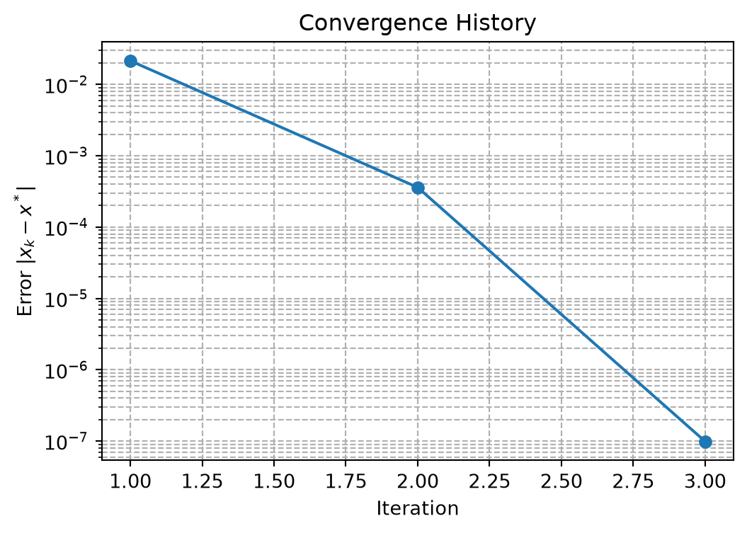
class RootFinder:
    def __init__(self, f, df=None):
        self.f = f
        self.df = df
        self.history = []

    def bisection(self, a, b, tol=1e-5, max_iter=100):
        self.history = []
        if self.f(a) * self.f(b) >= 0:
            raise ValueError("f(a) and f(b) must have opposite signs")
            
        for i in range(max_iter):
            c = (a + b) / 2.0
            self.history.append(c)
            
            if abs(self.f(c)) < tol or (b - a) / 2.0 < tol:
                return c
                
            if self.f(c) * self.f(a) < 0:
                b = c
            else:
                a = c
        return self.history[-1]

    def newton(self, x0, tol=1e-5, max_iter=100):
        if self.df is None:
            raise ValueError("Derivative df must be provided for Newton's method")
            
        self.history = [x0]
        x = x0
        for i in range(max_iter):
            fx = self.f(x)
            dfx = self.df(x)
            if dfx == 0:
                break
                
            x_new = x - fx / dfx
            self.history.append(x_new)
            
            if abs(x_new - x) < tol:
                return x_new
            x = x_new
        return x

    def plot_convergence(self):
        if not self.history:
            print("No history to plot.")
            return
            
        errors = [abs(self.history[i] - self.history[-1]) for i in range(len(self.history)-1)]
        
        plt.figure(figsize=(6, 4))
        plt.plot(range(1, len(errors)+1), errors, marker='o', linestyle='-')
        plt.yscale('log')
        plt.xlabel('Iteration')
        plt.ylabel('Error $|x_k - x^*|$')
        plt.title('Convergence History')
        plt.grid(True, which="both", ls="--")
        plt.show()

# Test the class
f = lambda x: x**3 - x - 2
df = lambda x: 3*x**2 - 1

finder = RootFinder(f, df)

root_bisect = finder.bisection(1, 2)
print(f"Bisection Root: {root_bisect}")

root_newton = finder.newton(1.5)
print(f"Newton Root: {root_newton}")

finder.plot_convergence()

Bisection Root: 1.5213851928710938
Newton Root: 1.5213797068045751

6 Practice Problems

1. Vectorization Practice: Create two arrays of size 1,000,000 using np.linspace. Calculate the Euclidean distance between them using a standard Python for loop and then using NumPy vectorization. Compare the computation times.
2. Taylor Series of Sine: Write a function my_sin(x, tol) that computes \(\sin(x)\) using its Taylor series around 0. The function should use a while loop that stops when the absolute value of the newly added term is less than tol.
3. Data I/O: Write a script that generates \(x\) and \(y\) data for \(y = e^{-x} \cos(2\\pi x)\), writes it to a CSV file without using Pandas (use built-in file I/O or np.savetxt), reads it back in, and plots it using Matplotlib.
4. Custom Plotting Function: Create a function plot_derivatives(f, x_range) that takes a mathematical function f and a NumPy array x_range. It should numerically approximate the first derivative \(f'(x)\) using central differences and plot both \(f(x)\) and \(f'(x)\) on the same graph with proper legends and axis labels.
5. Robust Root Finding: Extend the RootFinder class from the Hard example to include the Secant Method, which does not require the user to provide an exact analytical derivative.

7 Summary

Module Summary

• Python and NumPy: Python is highly readable, but loops are slow. NumPy provides vectorization, allowing for high-performance element-wise operations on arrays.
• Matplotlib: Essential for visualizing numerical behavior (e.g., error decay, function shapes). Use subplots to compare multiple views.
• Iteration and Convergence: Numerical methods often rely on loops. Always pair a while loop with a tolerance check (\(|x_{k+1} - x_k| < \\epsilon\)) and a maximum iteration limit.
• Code Modularity: Organize algorithms into reusable functions or classes. Document them heavily. Pass parameters explicitly (avoid global variables).

← Back to Course Index