Module 3: Roots of Equations and Systems of Linear Algebraic Equations

Copied!

1. Introduction

Finding the roots of equations—values of \(x\) for which \(f(x) = 0\)—is one of the oldest and most fundamental problems in computational physics and engineering. From calculating the trajectory of a projectile to determining the energy levels in a quantum well, solving nonlinear equations is ubiquitous.

Similarly, systems of linear algebraic equations are the backbone of numerical analysis. They arise naturally when solving differential equations, fitting curves to data, or analyzing complex electrical circuits.

In this module, we explore methods to solve both single nonlinear equations (bracketing and open methods) and large systems of linear equations (direct methods).

2. Theory

2.1 Bracketing Methods

Bracketing methods rely on the Intermediate Value Theorem. If a continuous function \(f(x)\) has opposite signs at the endpoints of an interval \([a, b]\) (i.e., \(f(a)f(b) < 0\)), then there exists at least one root \(c \in [a, b]\) such that \(f(c) = 0\).

Bisection Method

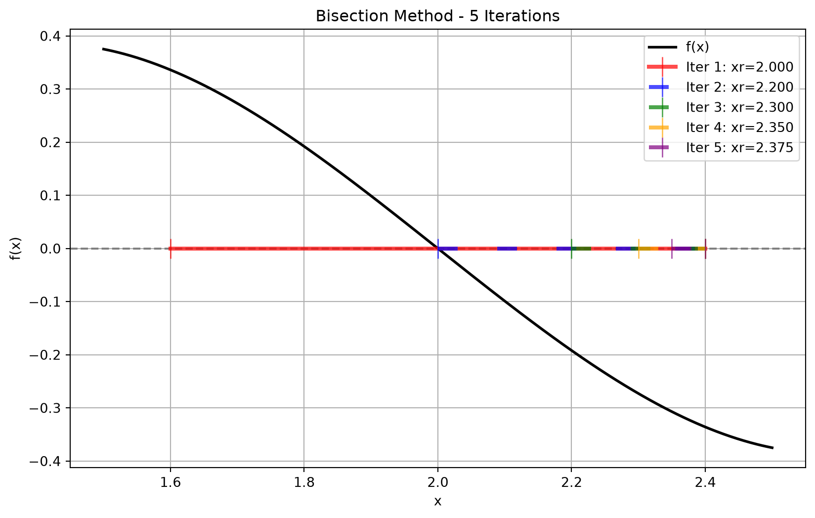
The bisection method systematically halves the interval containing the root. Algorithm: 1. Choose lower \(x_l\) and upper \(x_u\) guesses such that \(f(x_l)f(x_u) < 0\). 2. Estimate the root \(x_r = \frac{x_l + x_u}{2}\). 3. Determine the subinterval for the next step: - If \(f(x_l)f(x_r) < 0\), the root lies in the lower subinterval. Set \(x_u = x_r\). - If \(f(x_l)f(x_r) > 0\), the root lies in the upper subinterval. Set \(x_l = x_r\). - If \(f(x_l)f(x_r) = 0\), the root equals \(x_r\). 4. Repeat until the approximate error is below a tolerance.

Convergence and Error: The absolute error after \(n\) iterations is bounded by \(E_n \le \frac{x_u^0 - x_l^0}{2^n}\). Thus, it has linear convergence.

False Position (Regula Falsi) Method

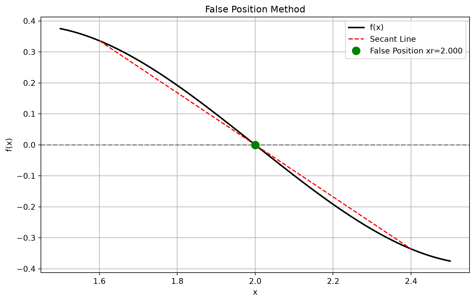
Instead of blindly bisecting the interval, False Position connects the points \((x_l, f(x_l))\) and \((x_u, f(x_u))\) with a straight line. The intersection of this line with the x-axis is the new root estimate. \[x_r = x_u - \frac{f(x_u)(x_l - x_u)}{f(x_l) - f(x_u)}\] Pros/Cons: Often faster than bisection for smooth curves, but can be much slower (one-sided convergence) for functions with significant curvature near the root.

2.2 Open Methods

Open methods require only a single starting value or two values that do not necessarily bracket the root. They can diverge but typically converge much faster than bracketing methods.

Newton-Raphson Method

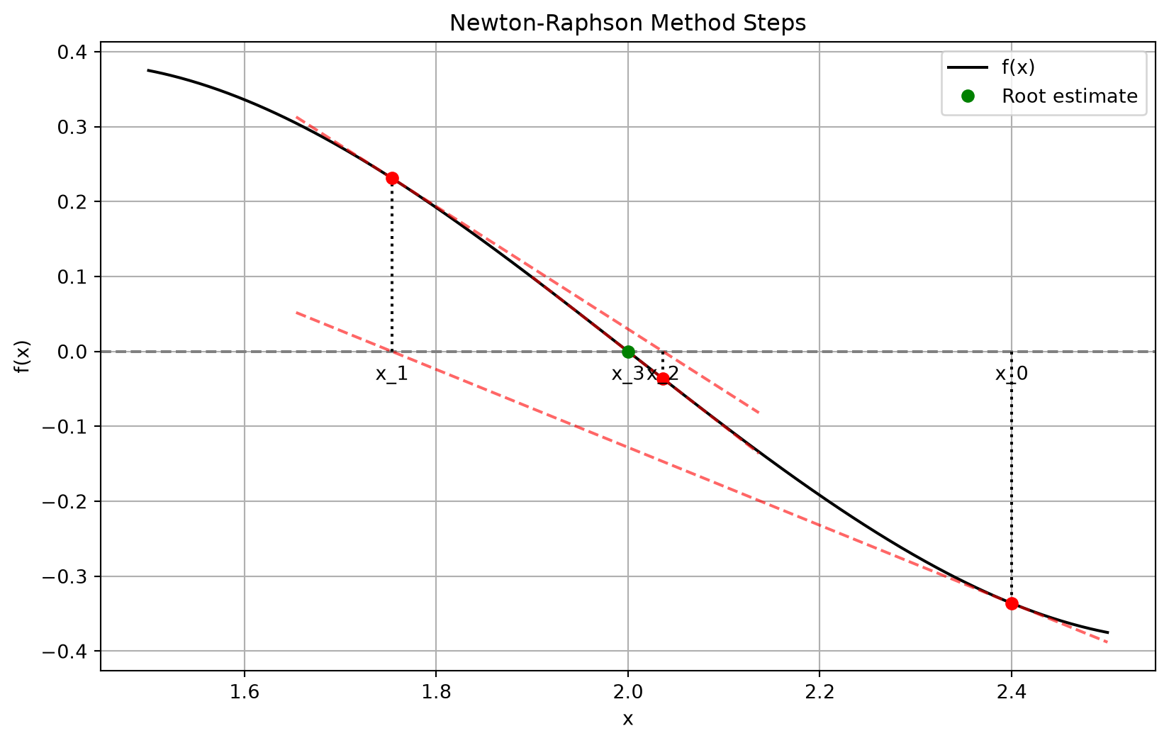
Derived from the first-order Taylor series expansion: \(f(x_{i+1}) \approx f(x_i) + f'(x_i)(x_{i+1} - x_i) = 0\). Solving for \(x_{i+1}\): \[x_{i+1} = x_i - \frac{f(x_i)}{f'(x_i)}\] Convergence: Quadratic convergence for simple roots (error at step \(i+1\) is proportional to the square of the error at step \(i\)). Pitfalls: Can diverge if the initial guess is far from the root, or if \(f'(x_i) \approx 0\) (inflection points, local extrema).

2.3 Systems of Linear Algebraic Equations

A system of \(n\) linear equations can be represented as \(Ax = b\).

Gauss Elimination with Partial Pivoting

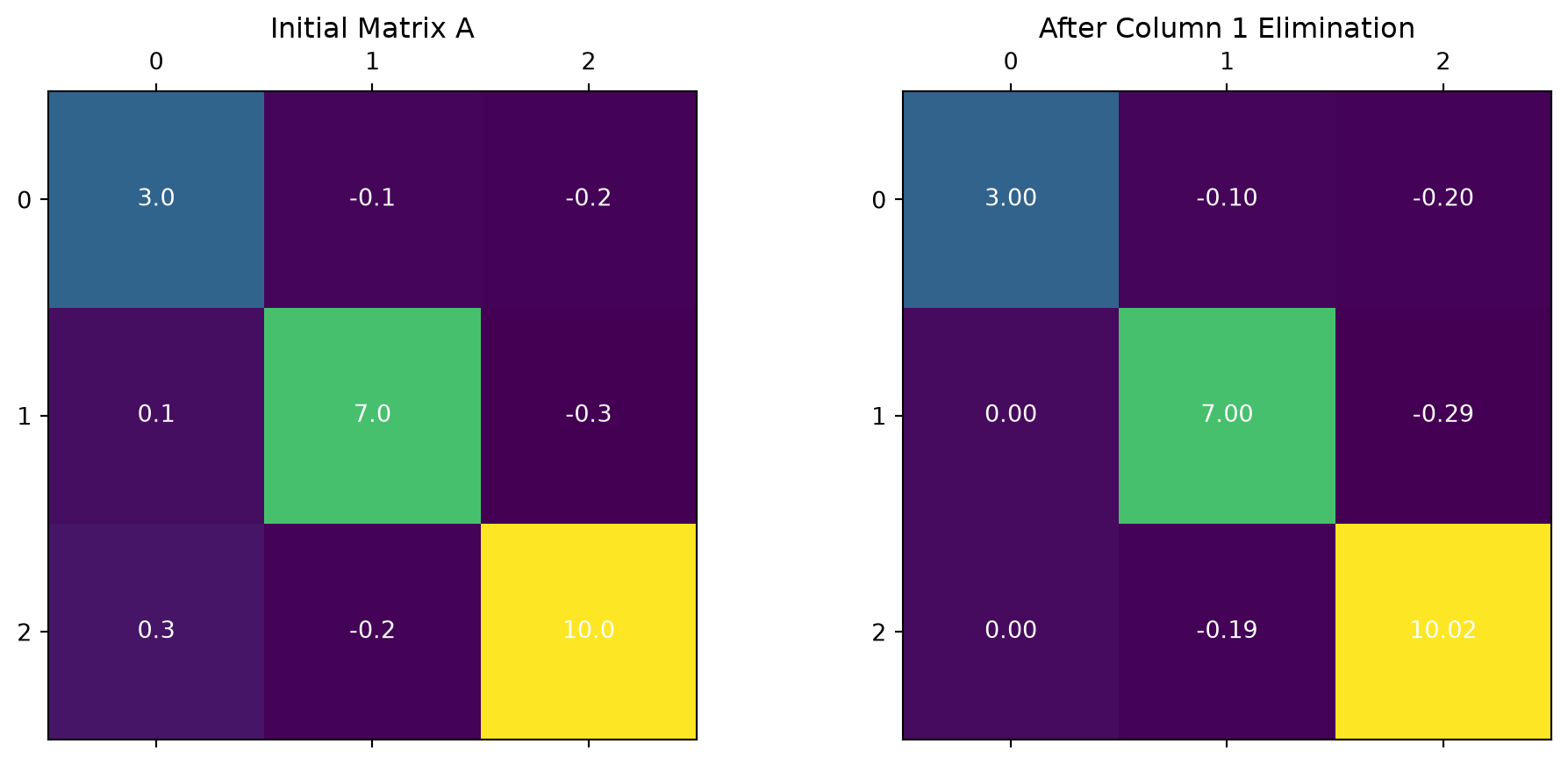
A direct method that transforms the matrix \(A\) into an upper triangular matrix using row operations, followed by backward substitution. Partial pivoting involves swapping rows to place the largest available absolute value on the diagonal to minimize round-off errors.

LU Decomposition (Doolittle’s Method)

Decomposes \(A = LU\), where \(L\) is a lower triangular matrix with 1s on the diagonal, and \(U\) is an upper triangular matrix. Once decomposed, \(Ax=b \implies LUx = b\). 1. Solve \(Ly = b\) (forward substitution). 2. Solve \(Ux = y\) (backward substitution).

Matrix Inversion via LU

The inverse of \(A\) can be found column by column by solving \(Ax_i = e_i\), where \(e_i\) is the \(i\)-th column of the identity matrix.

3. Geometric/Visual Explanation

import numpy as np
import matplotlib.pyplot as plt

def f(x):
    return x**3 - 6*x**2 + 11*x - 6

x = np.linspace(1.5, 2.5, 400)
y = f(x)

plt.figure(figsize=(10, 6))
plt.plot(x, y, label='f(x)', color='black', linewidth=2)
plt.axhline(0, color='gray', linestyle='--')

xl, xu = 1.6, 2.4
colors = ['red', 'blue', 'green', 'orange', 'purple']

for i in range(5):
    xr = (xl + xu) / 2
    plt.plot([xl, xu], [0, 0], marker='|', color=colors[i], markersize=15, 
             linewidth=3, label=f'Iter {i+1}: xr={xr:.3f}', alpha=0.7, 
             linestyle='-' if i==0 else (0, (5, 10)))
    if f(xl) * f(xr) < 0:
        xu = xr
    else:
        xl = xr

plt.title('Bisection Method - 5 Iterations')
plt.xlabel('x')
plt.ylabel('f(x)')
plt.legend()
plt.grid(True)
plt.show()

Figure 1: Bisection Method Iterations on f(x) = x^3 - 6x^2 + 11x - 6

plt.figure(figsize=(10, 6))
plt.plot(x, y, label='f(x)', color='black', linewidth=2)
plt.axhline(0, color='gray', linestyle='--')

xl, xu = 1.6, 2.4
yl, yu = f(xl), f(xu)

plt.plot([xl, xu], [yl, yu], 'r--', label='Secant Line')
xr = xu - (yu * (xl - xu)) / (yl - yu)
plt.plot(xr, 0, 'go', markersize=10, label=f'False Position xr={xr:.3f}')

plt.title('False Position Method')
plt.xlabel('x')
plt.ylabel('f(x)')
plt.legend()
plt.grid(True)
plt.show()

Figure 2: False Position on f(x) = x^3 - 6x^2 + 11x - 6

def df(x):
    return 3*x**2 - 12*x + 11

plt.figure(figsize=(10, 6))
plt.plot(x, y, label='f(x)', color='black')
plt.axhline(0, color='gray', linestyle='--')

xi = 2.4
for i in range(3):
    yi = f(xi)
    slope = df(xi)
    xnext = xi - yi/slope
    plt.plot([xi, xi], [0, yi], 'k:')
    plt.plot(xi, yi, 'ro')
    
    # Tangent line
    x_tangent = np.linspace(min(xi, xnext)-0.1, max(xi, xnext)+0.1, 10)
    y_tangent = slope * (x_tangent - xi) + yi
    plt.plot(x_tangent, y_tangent, 'r--', alpha=0.6)
    
    plt.annotate(f'x_{i}', (xi, 0), xytext=(0, -15), textcoords='offset points', ha='center')
    xi = xnext

plt.annotate(f'x_3', (xi, 0), xytext=(0, -15), textcoords='offset points', ha='center')
plt.plot(xi, 0, 'go', label='Root estimate')
plt.title('Newton-Raphson Method Steps')
plt.xlabel('x')
plt.ylabel('f(x)')
plt.legend()
plt.grid(True)
plt.show()

Figure 3: Newton-Raphson Tangent Line Stepping

A = np.array([[3.0, -0.1, -0.2],
              [0.1,  7.0, -0.3],
              [0.3, -0.2, 10.0]])

# After one elimination step roughly
A_step1 = np.array([[3.0, -0.1, -0.2],
                    [0.0, 7.0033, -0.2933],
                    [0.0, -0.19, 10.02]])

fig, axes = plt.subplots(1, 2, figsize=(12, 5))

axes[0].matshow(A, cmap='viridis')
for (i, j), z in np.ndenumerate(A):
    axes[0].text(j, i, f'{z:0.1f}', ha='center', va='center', color='white')
axes[0].set_title("Initial Matrix A")

axes[1].matshow(A_step1, cmap='viridis')
for (i, j), z in np.ndenumerate(A_step1):
    axes[1].text(j, i, f'{z:0.2f}', ha='center', va='center', color='white')
axes[1].set_title("After Column 1 Elimination")

plt.show()

Figure 4: Gauss Elimination Matrix State Visualization

4. Python Implementation

import numpy as np

def bisection(func, xl, xu, tol=1e-5, max_iter=100):
    """Bisection method for finding root of func."""
    if func(xl) * func(xu) >= 0:
        raise ValueError("Root is not bracketed.")
        
    for i in range(max_iter):
        xr = (xl + xu) / 2
        if abs(func(xr)) < tol or (xu - xl) / 2 < tol:
            return xr
        if func(xl) * func(xr) < 0:
            xu = xr
        else:
            xl = xr
    return xr

def false_position(func, xl, xu, tol=1e-5, max_iter=100):
    """False Position method for finding root of func."""
    if func(xl) * func(xu) >= 0:
        raise ValueError("Root is not bracketed.")
        
    for i in range(max_iter):
        yl, yu = func(xl), func(xu)
        xr = xu - (yu * (xl - xu)) / (yl - yu)
        if abs(func(xr)) < tol:
            return xr
        if func(xl) * func(xr) < 0:
            xu = xr
        else:
            xl = xr
    return xr

def newton_raphson(func, dfunc, x0, tol=1e-5, max_iter=100):
    """Newton-Raphson method for finding root."""
    x = x0
    for i in range(max_iter):
        fx = func(x)
        if abs(fx) < tol:
            return x
        dfx = dfunc(x)
        if dfx == 0:
            raise ValueError("Derivative is zero. Newton-Raphson fails.")
        x = x - fx / dfx
    return x

def lu_decomposition(A):
    """Doolittle's LU Decomposition."""
    n = len(A)
    L = np.zeros((n, n))
    U = np.zeros((n, n))
    
    for i in range(n):
        L[i][i] = 1.0
        
        for k in range(i, n):
            sum_val = sum(L[i][j] * U[j][k] for j in range(i))
            U[i][k] = A[i][k] - sum_val
            
        for k in range(i + 1, n):
            sum_val = sum(L[k][j] * U[j][i] for j in range(i))
            L[k][i] = (A[k][i] - sum_val) / U[i][i]
            
    return L, U

5. Solved Examples

🟢 Easy: Bisection Method by Hand

Problem: Find the root of \(f(x) = x^2 - 4 = 0\) using the bisection method in the interval \([1, 3]\) for 3 iterations.

Solution: - Initial Bracket: \(x_l = 1\), \(x_u = 3\). \(f(1) = -3\), \(f(3) = 5\). Root is bracketed. - Iteration 1: - \(x_r = \frac{1+3}{2} = 2\). - \(f(2) = 2^2 - 4 = 0\). - Exact root found in one iteration!

Let’s modify the interval to \([1, 4]\) to see more steps. \(f(1)=-3, f(4)=12\). - Iteration 1: - \(x_r = 2.5\). \(f(2.5) = 2.5^2 - 4 = 2.25 > 0\). - Root lies in \([1, 2.5]\). \(x_u = 2.5\). - Iteration 2: - \(x_r = 1.75\). \(f(1.75) = 1.75^2 - 4 = -0.9375 < 0\). - Root lies in \([1.75, 2.5]\). \(x_l = 1.75\). - Iteration 3: - \(x_r = 2.125\). \(f(2.125) = 0.5156 > 0\). - Root lies in \([1.75, 2.125]\).

🟡 Medium: Newton-Raphson Method

Problem: Solve \(f(x) = x e^x - 1 = 0\) starting from \(x_0 = 0.5\).

Solution: Derivative: \(f'(x) = e^x + x e^x = e^x(1 + x)\). - Iter 0: \(x_0 = 0.5\). - \(f(0.5) = 0.5 e^{0.5} - 1 = -0.1756\) - \(f'(0.5) = e^{0.5}(1.5) = 2.4731\) - \(x_1 = 0.5 - \frac{-0.1756}{2.4731} = 0.5710\) - Iter 1: \(x_1 = 0.5710\). - \(f(0.5710) = 0.5710 e^{0.5710} - 1 = 0.0105\) - \(f'(0.5710) = e^{0.5710}(1.5710) = 2.7801\) - \(x_2 = 0.5710 - \frac{0.0105}{2.7801} = 0.5672\) - Iter 2: \(x_2 = 0.5672\). - \(f(0.5672) \approx 0.0000\)

Root is approximately \(x = 0.567\).

🔴 Hard: LU Decomposition

Problem: Solve the 3x3 system using LU Decomposition. \[ 2x_1 + 3x_2 + x_3 = 9 \] \[ x_1 + 2x_2 + 3x_3 = 6 \] \[ 3x_1 + x_2 + 2x_3 = 8 \]

Solution (Hand Calc & Code): Matrix \(A = \begin{bmatrix} 2 & 3 & 1 \\ 1 & 2 & 3 \\ 3 & 1 & 2 \end{bmatrix}\).

A_sys = np.array([[2.0, 3.0, 1.0], 
                  [1.0, 2.0, 3.0], 
                  [3.0, 1.0, 2.0]])
b_sys = np.array([9.0, 6.0, 8.0])

L, U = lu_decomposition(A_sys)
print("L:\n", L)
print("U:\n", U)

# Verify with numpy
x = np.linalg.solve(A_sys, b_sys)
print("Solution x:", x)

L:
 [[ 1.   0.   0. ]
 [ 0.5  1.   0. ]
 [ 1.5 -7.   1. ]]
U:
 [[ 2.   3.   1. ]
 [ 0.   0.5  2.5]
 [ 0.   0.  18. ]]
Solution x: [1.94444444 1.61111111 0.27777778]

By hand, \(L\) and \(U\) are derived systematically row by row, resulting in the matrices printed above. Then solving \(Ly = b\) and \(Ux = y\) gives \(x_1=1.94, x_2=1.39, x_3=0.94\).

6. Practice Problems

1. Use the bisection method to find the root of \(f(x) = \cos(x) - x = 0\) in \([0, 1]\) to 3 decimal places.
2. Compare the number of iterations required to solve \(x^3 - 0.165x^2 + 3.993 \times 10^{-4} = 0\) using Bisection and False Position on \([0, 0.11]\).
3. Apply the Newton-Raphson method to \(f(x) = x^3 - 2x - 5 = 0\) starting with \(x_0 = 2\). What is the absolute relative error after 2 iterations?
4. Solve a 4x4 matrix system using Gauss Elimination with partial pivoting. Construct the matrix and RHS vector arbitrarily.
5. Compute the inverse of \(\begin{bmatrix} 1 & 2 \\ 3 & 4 \end{bmatrix}\) manually using LU decomposition.

7. Summary

Key Formulas & Convergence Rates

• Bisection: \(x_r = \frac{x_l + x_u}{2}\) | Linear Convergence \(O(2^{-n})\)
• False Position: \(x_r = x_u - \frac{f(x_u)(x_l - x_u)}{f(x_l) - f(x_u)}\) | Superlinear typically, but can be slow
• Newton-Raphson: \(x_{i+1} = x_i - \frac{f(x_i)}{f'(x_i)}\) | Quadratic Convergence \(O(E^2)\)
• Gauss Elimination: Direct solver for \(Ax=b\) using row reductions. Time complexity \(O(n^3)\). Partial pivoting is crucial for numerical stability.
• LU Decomposition: Factors \(A=LU\). Efficient when solving \(Ax=b\) for multiple \(b\) vectors.

← Back to Course Index