Module 4: System of Nonlinear Equations

Introduction

In physical sciences and engineering, we frequently encounter equations that do not adhere to the simple \(Ax = b\) form of linear systems. Nonlinearities arise naturally in systems with interacting components, relativistic corrections, orbital mechanics, and fluid dynamics. Unlike linear systems, which typically have a single unique solution, nonlinear systems can have multiple isolated roots, making their numerical resolution both fascinating and challenging.

This module explores the numerical techniques used to find roots of nonlinear equations, extending from single-variable functions to systems of multiple nonlinear equations. We will revisit the Bisection method, formally study Fixed-Point Iterations, and generalize Newton’s Method to multi-dimensional spaces using the Jacobian matrix.

Theory

1. What Makes Nonlinear Equations Different?

A linear system obeys the principle of superposition and can be represented via a constant matrix. A nonlinear system, however, takes the form: \[ \mathbf{F}(\mathbf{x}) = \mathbf{0} \] where \(\mathbf{x} = [x_1, x_2, \dots, x_n]^T\) and \(\mathbf{F}(\mathbf{x}) = [f_1(\mathbf{x}), f_2(\mathbf{x}), \dots, f_n(\mathbf{x})]^T\). Small changes in inputs can lead to disproportionate changes in outputs. There is no direct analytical way (like Gaussian elimination) to solve a general nonlinear system; thus, iterative methods are strictly necessary.

2. Bisection Method (Single Variable Recap)

For a single equation \(f(x) = 0\), if \(f(x)\) is continuous on an interval \([a, b]\) and \(f(a)f(b) < 0\), the Intermediate Value Theorem guarantees at least one root in \((a, b)\). The Bisection method systematically halves the interval: \[ c = \frac{a + b}{2} \] Replacing either \(a\) or \(b\) with \(c\) based on the sign of \(f(c)\). It is slow (linear convergence) but unconditionally stable and guaranteed to converge.

3. Fixed-Point Iteration Method

Any equation \(f(x) = 0\) can be rewritten in the form \(x = g(x)\). A solution \(x^*\) to this is called a fixed point. The iterative scheme is simply: \[ x_{n+1} = g(x_n) \]

Convergence and Lipschitz Condition

According to the Fixed-Point Theorem, if \(g(x)\) is continuous on \([a, b]\), \(g(x) \in [a,b]\) for all \(x \in [a,b]\), and it satisfies the Lipschitz condition with constant \(L < 1\) (i.e., \(|g'(x)| \le L < 1\)), the iteration will converge to a unique fixed point. The convergence rate depends heavily on \(g'(x^*)\).

4. Newton’s Method for Systems of Nonlinear Equations

For a single variable, Newton-Raphson iteration is \(x_{n+1} = x_n - \frac{f(x_n)}{f'(x_n)}\). To extend this to a system \(\mathbf{F}(\mathbf{x}) = \mathbf{0}\), we use the multi-dimensional Taylor series expansion. The derivative \(f'(x)\) is replaced by the Jacobian Matrix, \(J(\mathbf{x})\), whose elements are: \[ J_{ij} = \frac{\partial f_i}{\partial x_j} \] The iterative update becomes: \[ \mathbf{x}^{(k+1)} = \mathbf{x}^{(k)} - J(\mathbf{x}^{(k)})^{-1} \mathbf{F}(\mathbf{x}^{(k)}) \] In practice, we do not invert the Jacobian directly. Instead, we solve the linear system: \[ J(\mathbf{x}^{(k)}) \Delta \mathbf{x}^{(k)} = -\mathbf{F}(\mathbf{x}^{(k)}) \] and then update: \[ \mathbf{x}^{(k+1)} = \mathbf{x}^{(k)} + \Delta \mathbf{x}^{(k)} \]

5. Comparison of Convergence Rates

Bisection: Linear convergence. Error at step \(k+1\) is exactly \(E_{k+1} = 0.5 E_k\).
Fixed-Point: Linear convergence (usually), \(E_{k+1} \approx |g'(x^*)| E_k\).
Newton’s Method: Quadratic convergence near the root, \(E_{k+1} \approx C E_k^2\). The number of correct digits approximately doubles with each step, provided the initial guess is close enough.

Geometric / Visual Explanation

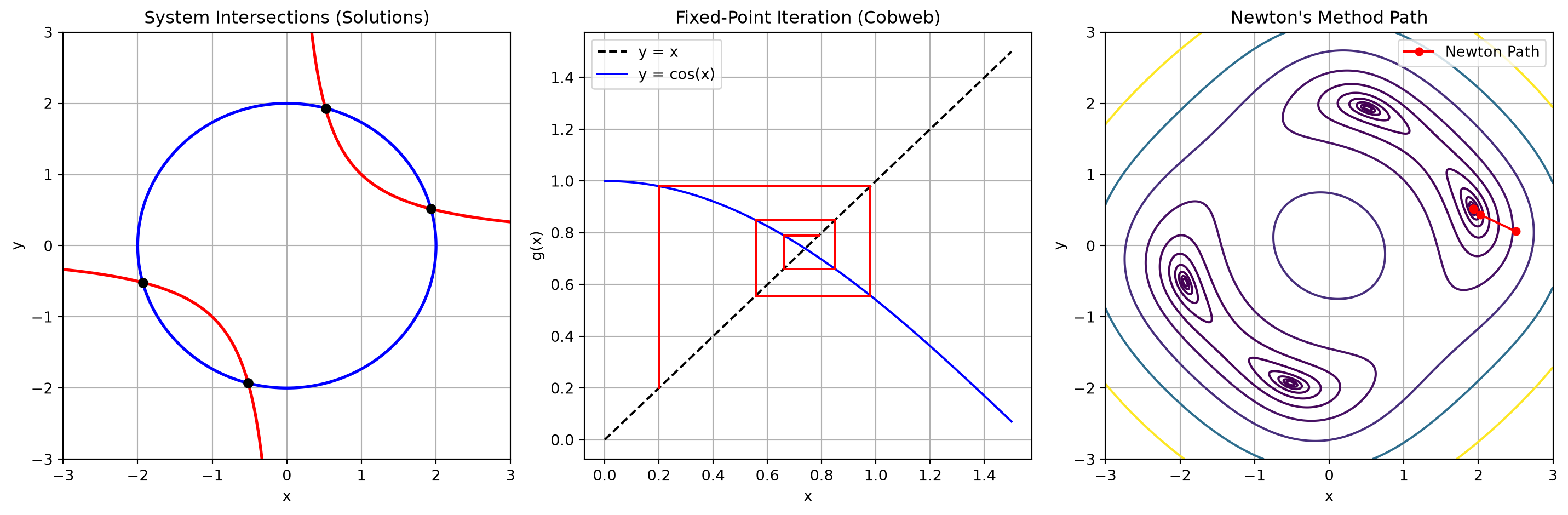
Let’s visualize the geometry of these methods using Python.

import numpy as np
import matplotlib.pyplot as plt

plt.figure(figsize=(15, 5))

# 1. Contour plot of two nonlinear equations
plt.subplot(1, 3, 1)
x = np.linspace(-3, 3, 400)
y = np.linspace(-3, 3, 400)
X, Y = np.meshgrid(x, y)
F1 = X**2 + Y**2 - 4
F2 = X * Y - 1
plt.contour(X, Y, F1, levels=[0], colors='blue', linewidths=2)
plt.contour(X, Y, F2, levels=[0], colors='red', linewidths=2)
plt.plot([1.93, -1.93, 0.52, -0.52], [0.52, -0.52, 1.93, -1.93], 'ko')
plt.title("System Intersections (Solutions)")
plt.xlabel("x")
plt.ylabel("y")
plt.grid(True)

# 2. Fixed-point iteration cobweb (staircase)
plt.subplot(1, 3, 2)
def g(x): return np.cos(x)
x_vals = np.linspace(0, 1.5, 100)
plt.plot(x_vals, x_vals, 'k--', label="y = x")
plt.plot(x_vals, g(x_vals), 'b-', label="y = cos(x)")
xi = 0.2
for _ in range(5):
    yi = g(xi)
    plt.plot([xi, xi], [xi, yi], 'r-')
    plt.plot([xi, yi], [yi, yi], 'r-')
    xi = yi
plt.title("Fixed-Point Iteration (Cobweb)")
plt.xlabel("x")
plt.ylabel("g(x)")
plt.legend()
plt.grid(True)

# 3. Newton's Method Convergence Path
plt.subplot(1, 3, 3)
plt.contour(X, Y, F1**2 + F2**2, levels=np.logspace(-2, 2, 10), cmap='viridis')
# Simple Newton path implementation for tracing
def newton_step(x, y):
    J = np.array([[2*x, 2*y], [y, x]])
    F = np.array([x**2 + y**2 - 4, x*y - 1])
    delta = np.linalg.solve(J, -F)
    return x + delta[0], y + delta[1]

px, py = 2.5, 0.2 # initial guess
path_x, path_y = [px], [py]
for _ in range(5):
    px, py = newton_step(px, py)
    path_x.append(px)
    path_y.append(py)

plt.plot(path_x, path_y, 'r-o', markersize=5, label="Newton Path")
plt.title("Newton's Method Path")
plt.xlabel("x")
plt.ylabel("y")
plt.legend()
plt.grid(True)

plt.tight_layout()
plt.show()

Figure 1: Visualizing Nonlinear Systems and Convergence Paths

Python Implementation

Below is a robust Python implementation of the numerical methods discussed.

import numpy as np

def bisection(f, a, b, tol=1e-6, max_iter=100):
    if f(a) * f(b) >= 0:
        raise ValueError("f(a) and f(b) must have opposite signs.")
    
    for i in range(max_iter):
        c = (a + b) / 2.0
        if abs(f(c)) < tol or (b - a) / 2.0 < tol:
            return c, i + 1
        
        if f(c) * f(a) < 0:
            b = c
        else:
            a = c
    return (a + b) / 2.0, max_iter

def fixed_point_iteration(g, x0, tol=1e-6, max_iter=100):
    x = x0
    for i in range(max_iter):
        x_new = g(x)
        if abs(x_new - x) < tol:
            return x_new, i + 1
        x = x_new
    raise Exception("Fixed-point iteration did not converge.")

def newton_system(F, J, x0, tol=1e-6, max_iter=100):
    x = np.array(x0, dtype=float)
    for i in range(max_iter):
        Fx = F(x)
        Jx = J(x)
        if np.linalg.norm(Fx) < tol:
            return x, i
        
        delta = np.linalg.solve(Jx, -Fx)
        x = x + delta
        
        if np.linalg.norm(delta) < tol:
            return x, i + 1
            
    raise Exception("Newton's method did not converge.")

Solved Examples

🟢 Easy: Fixed-Point Iteration

Problem: Solve \(x^3 - x - 1 = 0\) using fixed-point iteration.

Solution: Rewrite as \(x = (x + 1)^{1/3}\). Let \(g(x) = (x + 1)^{1/3}\). Using initial guess \(x_0 = 1.0\): - \(x_1 = (1.0 + 1)^{1/3} = 1.2599\) - \(x_2 = (1.2599 + 1)^{1/3} = 1.3123\) - \(x_3 = (1.3123 + 1)^{1/3} = 1.3224\) - \(x_4 = (1.3224 + 1)^{1/3} = 1.3243\) Converges to \(x^* \approx 1.3247\).

🟡 Medium: Newton’s Method for Systems

Problem: Solve \(x^2 + y^2 = 4\) and \(xy = 1\) using Newton’s method with initial guess \((2, 0.5)\).

Solution: Define \(\mathbf{F}(x,y) = [x^2 + y^2 - 4, xy - 1]^T\). Jacobian \(J(x,y) = \begin{bmatrix} 2x & 2y \\ y & x \end{bmatrix}\).

Iteration 1: \(\mathbf{x}^{(0)} = [2, 0.5]^T\) \(\mathbf{F}(\mathbf{x}^{(0)}) = [0.25, 0]^T\) \(J(\mathbf{x}^{(0)}) = \begin{bmatrix} 4 & 1 \\ 0.5 & 2 \end{bmatrix}\) Solve \(J \Delta \mathbf{x} = -\mathbf{F} \implies \Delta \mathbf{x} = [-0.0667, 0.0167]^T\). Update: \(\mathbf{x}^{(1)} = [1.9333, 0.5167]^T\). True solution: \(x \approx 1.93185, y \approx 0.51764\).

🔴 Hard: Convergence Rates Comparison

Problem: Solve \(\sin(x) - x/2 = 0\) starting near \(x = 2\), and compare iterations for Bisection, Fixed-Point, and Newton’s.

Solution: True root \(x^* \approx 1.895494\). 1. Bisection: Interval \([1.5, 2.5]\), tol \(10^{-6}\). Takes \(\sim 20\) iterations. 2. Fixed-Point: \(g(x) = 2\sin(x)\), \(x_0 = 2.0\). Takes \(\sim 15\) iterations. 3. Newton: \(x_{n+1} = x_n - \frac{\sin(x_n) - x_n/2}{\cos(x_n) - 0.5}\). From \(x_0=2.0\), converges to \(10^{-6}\) in just 3 iterations!

Practice Problems

Apply the Bisection method to \(f(x) = 1/x\) on \([-1, 1]\). Why is this problematic?
For \(x^2 - x - 2 = 0\), test \(g_1(x) = x^2 - 2\) and \(g_2(x) = \sqrt{x+2}\). Which converges for \(x_0 > 0\)?
Formulate the Jacobian for \(e^x - y = 0\) and \(xy - e^y = 0\).
Calculate the Lipschitz constant for \(g(x) = e^{-x}\) on \([0, 1]\).
Use Python to find the intersection of \(x^2/4 + y^2/9 = 1\) and \(x^2 - y^2 = 1\).

Summary

Module 4 Summary

Nonlinear Equations require iterative numerical methods.
Bisection Method: Robust but slow linear convergence.
Fixed-Point Iteration: \(x=g(x)\). Converges linearly if \(|g'(x)| < 1\).
Newton’s Method for Systems: Generalizes using the Jacobian Matrix. Achieves quadratic convergence but requires a good initial guess and solving a linear system at each step.

← Back to Course Index