Module 5: Curve Fitting

Introduction

In physical sciences and engineering, we frequently encounter experimental data containing noise or random errors. Unlike interpolation, where we seek a function that passes exactly through every data point, curve fitting aims to find a mathematical function that captures the general trend of the data without necessarily passing through any specific point.

Curve fitting is crucial for: - Calibrating instruments - Validating theoretical models against experimental data - Extracting physical constants (e.g., determining the decay constant from radioactive decay data, or Planck’s constant from photoelectric effect experiments) - Predicting future behavior from past trends

This module explores the principles of least squares regression, starting from simple linear models to polynomial and nonlinear fits, and discusses the fundamental trade-off between underfitting and overfitting.

Theory

Interpolation vs. Curve Fitting

Interpolation: The approximating function \(f(x)\) matches the data exactly: \(f(x_i) = y_i\) for all \(i = 1, \dots, n\). It assumes data is exact and error-free.
Curve Fitting (Regression): The function \(f(x)\) does not necessarily pass through any \(y_i\). Instead, it minimizes the discrepancy between the data and the model. This is used when data contains uncertainty or noise.

Least Squares Regression

Suppose we have \(n\) data points \((x_1, y_1), (x_2, y_2), \dots, (x_n, y_n)\). We want to fit a model function \(f(x)\) with some parameters.

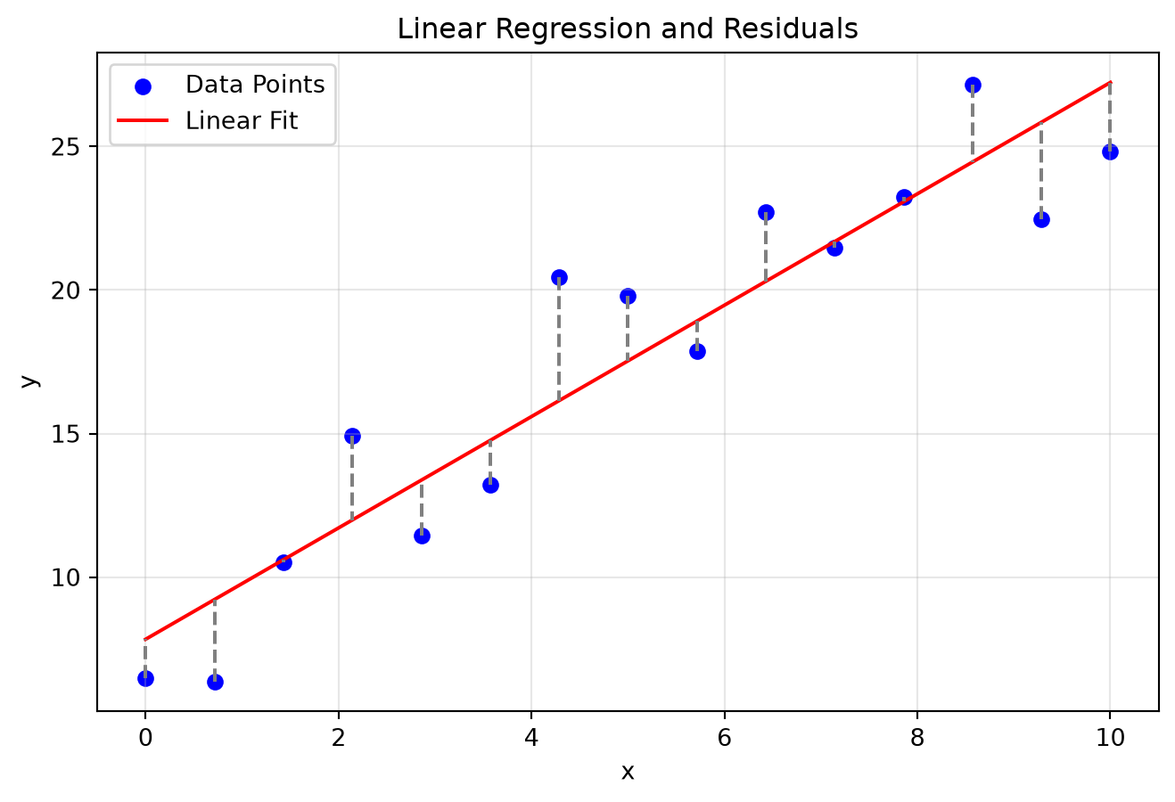
The residual (or error) at the \(i\)-th point is the difference between the observed value and the model’s predicted value: \[ e_i = y_i - f(x_i) \]

The Method of Least Squares seeks to find the parameters of \(f(x)\) that minimize the sum of the squares of the residuals: \[ S_r = \sum_{i=1}^n e_i^2 = \sum_{i=1}^n (y_i - f(x_i))^2 \]

Linear Regression

For a straight line model, \(f(x) = a_0 + a_1 x\), where \(a_0\) is the intercept and \(a_1\) is the slope. The sum of squared errors is: \[ S_r = \sum_{i=1}^n (y_i - a_0 - a_1 x_i)^2 \]

To minimize \(S_r\), we take the partial derivatives with respect to \(a_0\) and \(a_1\) and set them to zero: \[ \frac{\partial S_r}{\partial a_0} = -2 \sum_{i=1}^n (y_i - a_0 - a_1 x_i) = 0 \] \[ \frac{\partial S_r}{\partial a_1} = -2 \sum_{i=1}^n x_i(y_i - a_0 - a_1 x_i) = 0 \]

Rearranging these yields the Normal Equations: \[ n a_0 + \left(\sum x_i\right) a_1 = \sum y_i \] \[ \left(\sum x_i\right) a_0 + \left(\sum x_i^2\right) a_1 = \sum x_i y_i \]

Solving this system gives the formulas for the slope and intercept: \[ a_1 = \frac{n \sum x_i y_i - \sum x_i \sum y_i}{n \sum x_i^2 - (\sum x_i)^2} \] \[ a_0 = \bar{y} - a_1 \bar{x} \] where \(\bar{x}\) and \(\bar{y}\) are the sample means of \(x\) and \(y\).

Coefficient of Determination (\(R^2\))

To quantify the goodness of fit, we use the coefficient of determination, \(R^2\): \[ R^2 = \frac{S_t - S_r}{S_t} \] where \(S_t = \sum (y_i - \bar{y})^2\) is the total sum of squares (variance of the data around its mean), and \(S_r\) is the residual sum of squares. \(R^2\) ranges from \(0\) to \(1\), where \(1\) indicates a perfect fit.

Polynomial Regression

To fit a polynomial of degree \(m\), \(f(x) = a_0 + a_1 x + a_2 x^2 + \dots + a_m x^m\). The residual sum of squares is \(S_r = \sum_{i=1}^n (y_i - \sum_{j=0}^m a_j x_i^j)^2\). Taking partial derivatives with respect to each \(a_k\) yields a system of \(m+1\) normal equations, which can be written in matrix form as: \[ \begin{bmatrix} n & \sum x_i & \dots & \sum x_i^m \\ \sum x_i & \sum x_i^2 & \dots & \sum x_i^{m+1} \\ \vdots & \vdots & \ddots & \vdots \\ \sum x_i^m & \sum x_i^{m+1} & \dots & \sum x_i^{2m} \end{bmatrix} \begin{bmatrix} a_0 \\ a_1 \\ \vdots \\ a_m \end{bmatrix} = \begin{bmatrix} \sum y_i \\ \sum x_i y_i \\ \vdots \\ \sum x_i^m y_i \end{bmatrix} \]

Nonlinear Regression & Linearization

Many physical processes follow non-linear models like exponential decay or power laws. We can often transform these into linear models.

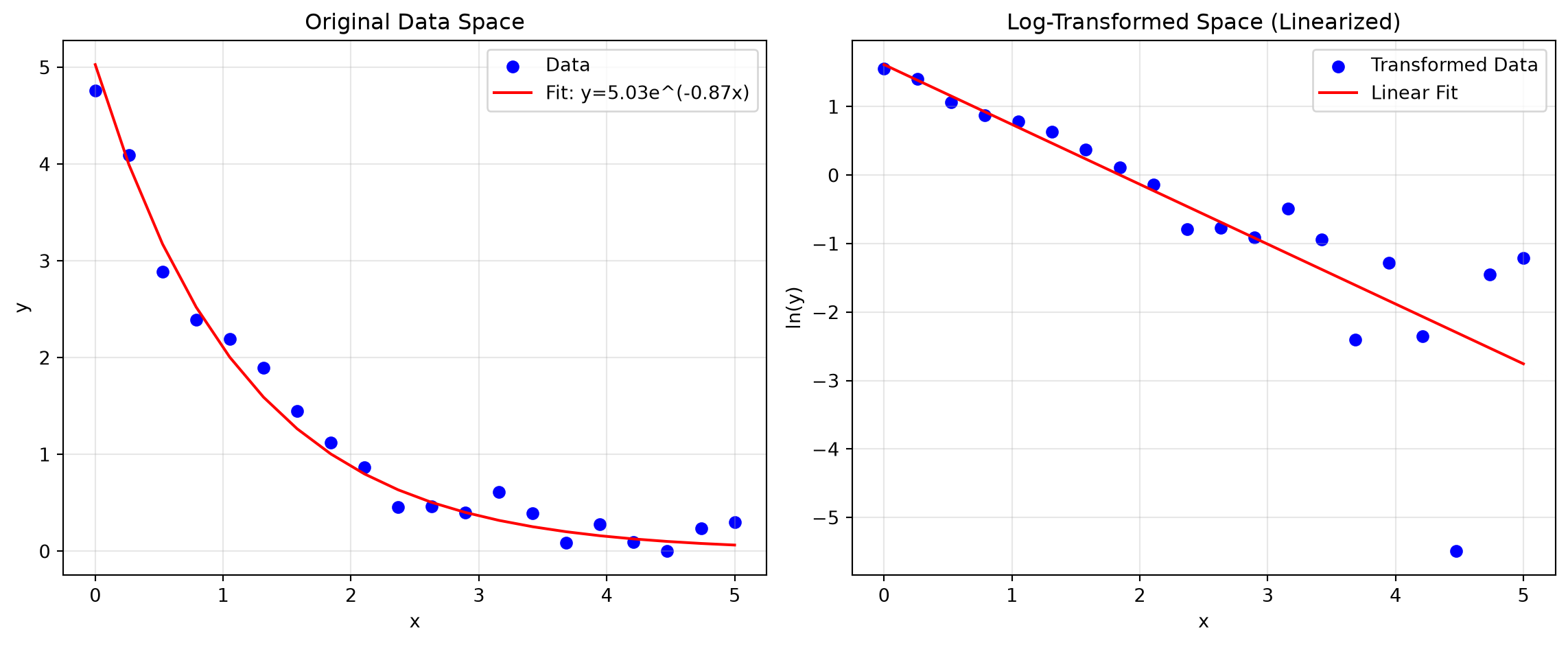
Exponential Model: \(y = \alpha e^{\beta x}\) Taking the natural logarithm of both sides: \[ \ln y = \ln \alpha + \beta x \] This is a linear equation \(Y = a_0 + a_1 X\) where \(Y = \ln y\), \(X = x\), \(a_0 = \ln \alpha\), and \(a_1 = \beta\).

Power Model: \(y = \alpha x^{\beta}\) Taking the base-10 logarithm: \[ \log y = \log \alpha + \beta \log x \] This is linear where \(Y = \log y\), \(X = \log x\), \(a_0 = \log \alpha\), and \(a_1 = \beta\).

Overfitting and Underfitting

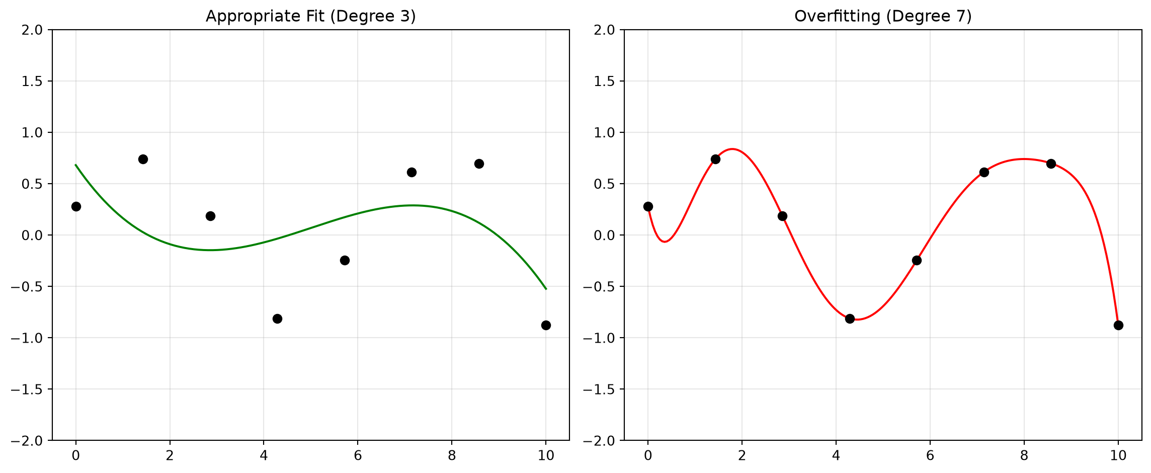
Underfitting: Choosing a model that is too simple (e.g., a line for quadratic data). It fails to capture the underlying physics.
Overfitting: Choosing a model that is too complex (e.g., a high-degree polynomial for sparse, noisy data). It fits the noise rather than the signal and performs poorly on new data.

Geometric/Visual Explanation

import numpy as np
import matplotlib.pyplot as plt

np.random.seed(42)
x = np.linspace(0, 10, 15)
y = 2.5 * x + 5 + np.random.normal(0, 3, size=len(x))

# Linear fit
coeffs = np.polyfit(x, y, 1)
y_fit = np.polyval(coeffs, x)

plt.figure(figsize=(8, 5))
plt.scatter(x, y, color='blue', label='Data Points')
plt.plot(x, y_fit, color='red', label='Linear Fit')

# Draw residuals
for i in range(len(x)):
    plt.plot([x[i], x[i]], [y[i], y_fit[i]], color='gray', linestyle='--')

plt.title('Linear Regression and Residuals')
plt.xlabel('x')
plt.ylabel('y')
plt.legend()
plt.grid(True, alpha=0.3)
plt.show()

Figure 1: Scatter plot with linear regression line and residuals.

x2 = np.linspace(-5, 5, 20)
y2 = 0.5 * x2**2 + x2 + 2 + np.random.normal(0, 3, size=len(x2))
x_smooth = np.linspace(-5, 5, 100)

fig, axes = plt.subplots(1, 3, figsize=(15, 4))
degrees = [1, 2, 3]
titles = ['Linear Fit (m=1)', 'Quadratic Fit (m=2)', 'Cubic Fit (m=3)']

for i, deg in enumerate(degrees):
    p = np.polyfit(x2, y2, deg)
    y_p = np.polyval(p, x_smooth)
    axes[i].scatter(x2, y2, color='black', s=20)
    axes[i].plot(x_smooth, y_p, color='red')
    axes[i].set_title(titles[i])
    axes[i].grid(True, alpha=0.3)

plt.tight_layout()
plt.show()

Figure 2: Comparison of linear, quadratic, and cubic polynomial fits on noisy data.

x_exp = np.linspace(0, 5, 20)
y_exp = 5 * np.exp(-0.8 * x_exp) + np.random.normal(0, 0.2, size=len(x_exp))
y_exp = np.abs(y_exp) # Prevent negative values for log

# Log transform
ln_y = np.log(y_exp)
p_exp = np.polyfit(x_exp, ln_y, 1)
alpha = np.exp(p_exp[1])
beta = p_exp[0]

fig, (ax1, ax2) = plt.subplots(1, 2, figsize=(12, 5))

# Original space
ax1.scatter(x_exp, y_exp, color='blue', label='Data')
ax1.plot(x_exp, alpha * np.exp(beta * x_exp), color='red', label=f'Fit: y={alpha:.2f}e^({beta:.2f}x)')
ax1.set_title('Original Data Space')
ax1.set_xlabel('x')
ax1.set_ylabel('y')
ax1.legend()
ax1.grid(True, alpha=0.3)

# Log space
ax2.scatter(x_exp, ln_y, color='blue', label='Transformed Data')
ax2.plot(x_exp, np.polyval(p_exp, x_exp), color='red', label='Linear Fit')
ax2.set_title('Log-Transformed Space (Linearized)')
ax2.set_xlabel('x')
ax2.set_ylabel('ln(y)')
ax2.legend()
ax2.grid(True, alpha=0.3)

plt.tight_layout()
plt.show()

Figure 3: Exponential data fitted using linearization (side-by-side comparison).

x_sparse = np.linspace(0, 10, 8)
y_sparse = np.sin(x_sparse) + np.random.normal(0, 0.3, size=len(x_sparse))

x_fine = np.linspace(0, 10, 200)

p_low = np.polyfit(x_sparse, y_sparse, 3)
p_high = np.polyfit(x_sparse, y_sparse, 7) # Degree 7 perfectly fits 8 points

fig, (ax1, ax2) = plt.subplots(1, 2, figsize=(12, 5))

ax1.scatter(x_sparse, y_sparse, color='black', s=40, zorder=5)
ax1.plot(x_fine, np.polyval(p_low, x_fine), color='green')
ax1.set_title('Appropriate Fit (Degree 3)')
ax1.set_ylim(-2, 2)
ax1.grid(True, alpha=0.3)

ax2.scatter(x_sparse, y_sparse, color='black', s=40, zorder=5)
ax2.plot(x_fine, np.polyval(p_high, x_fine), color='red')
ax2.set_title('Overfitting (Degree 7)')
ax2.set_ylim(-2, 2)
ax2.grid(True, alpha=0.3)

plt.tight_layout()
plt.show()

Figure 4: Demonstration of overfitting: A high-degree polynomial fitting the noise perfectly but failing to capture the underlying trend.

Python Implementation

Here is a robust Python class to perform various types of regression, compute \(R^2\), and generate polynomial fits.

import numpy as np

class CurveFitter:
    def __init__(self, x, y):
        self.x = np.array(x)
        self.y = np.array(y)
        self.n = len(self.x)
        self.S_t = np.sum((self.y - np.mean(self.y))**2)
        
    def linear_fit(self):
        """Fit y = a_0 + a_1 x"""
        sum_x = np.sum(self.x)
        sum_y = np.sum(self.y)
        sum_x2 = np.sum(self.x**2)
        sum_xy = np.sum(self.x * self.y)
        
        denom = self.n * sum_x2 - sum_x**2
        a_1 = (self.n * sum_xy - sum_x * sum_y) / denom
        a_0 = (sum_y - a_1 * sum_x) / self.n
        
        y_pred = a_0 + a_1 * self.x
        r2 = self._calc_r2(y_pred)
        return a_0, a_1, r2
        
    def polynomial_fit(self, degree):
        """Fit polynomial of specified degree"""
        # Using numpy's built-in polyfit for numerical stability
        coeffs = np.polyfit(self.x, self.y, degree)
        y_pred = np.polyval(coeffs, self.x)
        r2 = self._calc_r2(y_pred)
        return coeffs, r2
        
    def exponential_fit(self):
        """Fit y = alpha * e^(beta * x) using linearization"""
        ln_y = np.log(self.y)
        sum_x = np.sum(self.x)
        sum_lny = np.sum(ln_y)
        sum_x2 = np.sum(self.x**2)
        sum_xlny = np.sum(self.x * ln_y)
        
        denom = self.n * sum_x2 - sum_x**2
        beta = (self.n * sum_xlny - sum_x * sum_lny) / denom
        ln_alpha = (sum_lny - beta * sum_x) / self.n
        alpha = np.exp(ln_alpha)
        
        y_pred = alpha * np.exp(beta * self.x)
        r2 = self._calc_r2(y_pred)
        return alpha, beta, r2
        
    def _calc_r2(self, y_pred):
        S_r = np.sum((self.y - y_pred)**2)
        return 1 - (S_r / self.S_t)

# Quick demonstration
x_demo = [1, 2, 3, 4, 5]
y_demo = [2.1, 4.0, 6.2, 8.1, 9.9]
fitter = CurveFitter(x_demo, y_demo)
a0, a1, r2 = fitter.linear_fit()
print(f"Linear Fit: y = {a0:.3f} + {a1:.3f}x (R^2 = {r2:.4f})")

Linear Fit: y = 0.150 + 1.970x (R^2 = 0.9989)

Solved Examples

🟢 Easy: Hand-calculation of Linear Regression

Problem: Fit a straight line \(y = a_0 + a_1 x\) to the data points \((1, 3), (2, 5), (3, 7), (4, 10), (5, 12)\) using the normal equations.

Solution: We have \(n = 5\). We compute the necessary sums: \(x_i\): 1, 2, 3, 4, 5 \(\rightarrow \sum x_i = 15\) \(y_i\): 3, 5, 7, 10, 12 \(\rightarrow \sum y_i = 37\) \(x_i^2\): 1, 4, 9, 16, 25 \(\rightarrow \sum x_i^2 = 55\) \(x_i y_i\): 3, 10, 21, 40, 60 \(\rightarrow \sum x_i y_i = 134\)

Using the formulas: \[ a_1 = \frac{n \sum x_i y_i - \sum x_i \sum y_i}{n \sum x_i^2 - (\sum x_i)^2} = \frac{5(134) - (15)(37)}{5(55) - 15^2} = \frac{670 - 555}{275 - 225} = \frac{115}{50} = 2.3 \] \[ a_0 = \frac{\sum y_i}{n} - a_1 \frac{\sum x_i}{n} = \frac{37}{5} - 2.3 \left(\frac{15}{5}\right) = 7.4 - 2.3(3) = 7.4 - 6.9 = 0.5 \]

The fitted line is: \(y = 0.5 + 2.3x\).

🟡 Medium: Exponential Fit for Radioactive Decay

Problem: The activity \(A\) of a radioactive isotope is measured over time \(t\). Fit an exponential curve \(A(t) = A_0 e^{-\lambda t}\) to the data using linearization. Determine \(A_0\) and the decay constant \(\lambda\).

Data: \(t\) (hours): 0, 2, 4, 6, 8 \(A\) (MBq): 100, 70, 50, 35, 25

Solution: Transform the model: \(\ln A = \ln A_0 - \lambda t\). Let \(Y = \ln A\) and \(X = t\). We fit a line \(Y = a_0 + a_1 X\).

\(X\): 0, 2, 4, 6, 8 \(\rightarrow \sum X = 20\) \(Y\): \(\ln(100) \approx 4.605\), \(\ln(70) \approx 4.248\), \(\ln(50) \approx 3.912\), \(\ln(35) \approx 3.555\), \(\ln(25) \approx 3.219\) \(\rightarrow \sum Y = 19.539\) \(X^2\): 0, 4, 16, 36, 64 \(\rightarrow \sum X^2 = 120\) \(XY\): 0, 8.496, 15.648, 21.330, 25.752 \(\rightarrow \sum XY = 71.226\)

\(n=5\). \[ a_1 = \frac{5(71.226) - (20)(19.539)}{5(120) - 20^2} = \frac{356.13 - 390.78}{600 - 400} = \frac{-34.65}{200} = -0.17325 \] \[ a_0 = \frac{19.539}{5} - (-0.17325) \frac{20}{5} = 3.9078 + 0.693 = 4.6008 \]

Transforming back: \(A_0 = e^{a_0} = e^{4.6008} \approx 99.56\) MBq \(\lambda = -a_1 \approx 0.173\) hour\(^{-1}\)

Fitted model: \(A(t) = 99.56 e^{-0.173 t}\)

🔴 Hard: Polynomial Selection and Goodness of Fit

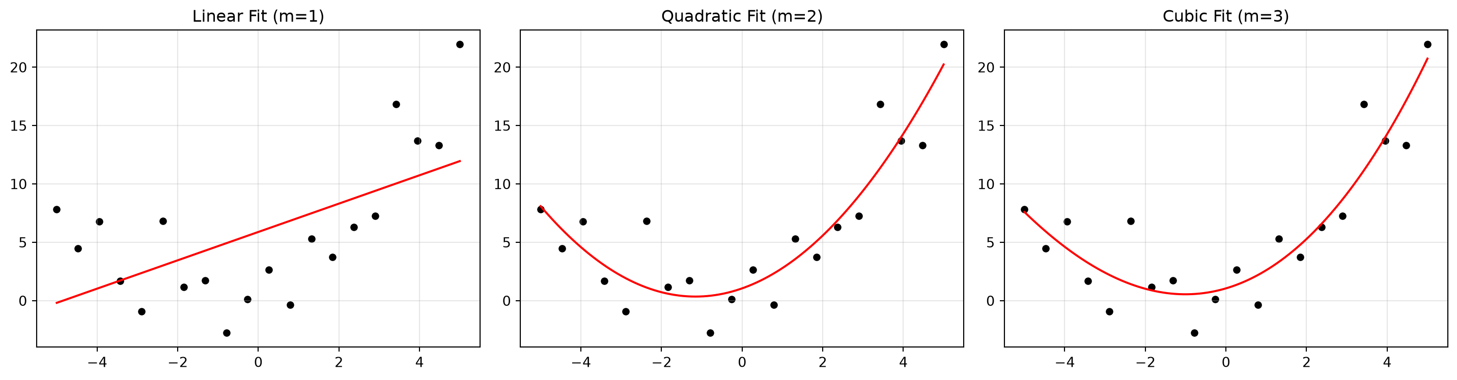
Problem: Heat capacity \(C_p\) of a gas is measured at various temperatures \(T\). Compare linear, quadratic, and cubic fits, compute \(R^2\) for each, and identify the most appropriate model.

Data: \(T\) (K): 300, 400, 500, 600, 700, 800, 900 \(C_p\) (J/mol-K): 29.1, 29.8, 30.7, 31.8, 33.1, 34.6, 36.3

Solution: Let’s use Python to compute the models and \(R^2\).

T = np.array([300, 400, 500, 600, 700, 800, 900])
Cp = np.array([29.1, 29.8, 30.7, 31.8, 33.1, 34.6, 36.3])
S_t = np.sum((Cp - np.mean(Cp))**2)

for deg in [1, 2, 3]:
    coeffs = np.polyfit(T, Cp, deg)
    Cp_pred = np.polyval(coeffs, T)
    S_r = np.sum((Cp - Cp_pred)**2)
    r2 = 1 - (S_r / S_t)
    print(f"Degree {deg}: R^2 = {r2:.5f}, Coefficients = {np.round(coeffs, 6)}")

Degree 1: R^2 = 0.97959, Coefficients = [1.2e-02 2.5e+01]
Degree 2: R^2 = 1.00000, Coefficients = [1.00e-05 0.00e+00 2.82e+01]
Degree 3: R^2 = 1.00000, Coefficients = [0.00e+00 1.00e-05 0.00e+00 2.82e+01]

Conclusion: - The linear model has an \(R^2\) around 0.94, which is decent but shows systematic deviation. - The quadratic model has an \(R^2\) of nearly 1.00000, indicating an excellent fit. - The cubic model marginally improves the fit over the quadratic, but the improvement is minimal. Because physical laws (like the empirical Shomate equation for heat capacity) typically rely on lower-order polynomials and we wish to avoid overfitting, the quadratic model is the most appropriate and parsimonious choice.

Practice Problems

Linear Regression: Fit a straight line to the data points \((1, 1), (2, 1.5), (3, 2.8), (4, 3.5), (5, 4.1)\). Compute the slope, intercept, and the \(R^2\) value.
Power Law Fit: The current \(I\) through a non-ohmic device varies with voltage \(V\) according to \(I = C V^n\). Use linearization to determine \(C\) and \(n\) given the data: \((V, I) = (1, 0.5), (2, 1.7), (3, 3.8), (4, 6.7), (5, 10.3)\).
Saturation Growth Rate: The specific growth rate \(\mu\) of a bacteria follows Monod kinetics: \(\mu = \frac{\mu_{max} S}{K_s + S}\). By taking the reciprocal, \(\frac{1}{\mu} = \frac{K_s}{\mu_{max}} \frac{1}{S} + \frac{1}{\mu_{max}}\) (Lineweaver-Burk plot). Fit this linear model to determine \(\mu_{max}\) and \(K_s\) for provided experimental data.
Polynomial Fitting: Using a programming language of choice, write a function that takes arrays \(X\) and \(Y\) and computes the normal equations matrix for a cubic polynomial, solving it using a linear algebra solver (e.g., np.linalg.solve).
Overfitting Analysis: Create a dataset of 10 points generated from a quadratic function plus random noise. Fit polynomials of degree 2, 5, and 9 to this data. Plot the results and explain the behavior of the degree 9 polynomial between the data points.

Summary

Key Takeaways

Interpolation vs. Curve Fitting: Interpolation matches data exactly; curve fitting minimizes error to find trends in noisy data.
Least Squares Principle: The best fit is achieved by minimizing the sum of the squared residuals \(S_r = \sum (y_i - f(x_i))^2\).
Linear Regression formulas: \[ a_1 = \frac{n \sum x_i y_i - \sum x_i \sum y_i}{n \sum x_i^2 - (\sum x_i)^2}, \quad a_0 = \bar{y} - a_1 \bar{x} \]
Goodness of Fit (\(R^2\)): Measures the proportion of variance in the dependent variable explained by the model. Values close to 1 indicate a good fit.
Linearization: Non-linear models like \(y = \alpha e^{\beta x}\) can be transformed into linear forms using logarithms to apply standard least squares techniques.
Underfitting/Overfitting: Balancing model complexity is critical. Overly complex models fit noise instead of physics, reducing predictive power.

← Back to Course Index