In experimental physics, computational fluid dynamics, and data analysis, we often collect discrete data points—measurements of a physical quantity (like temperature, velocity, or magnetic field) at specific spatial or temporal coordinates. However, to evaluate the function between these known data points or to approximate the underlying continuous physical process, we need Interpolation.
Interpolation is the mathematical technique of constructing a continuous function (often a polynomial) that passes exactly through a given set of discrete data points. Unlike curve fitting (which minimizes errors but doesn’t necessarily pass through the points), interpolation strictly honors the data. In this module, we will explore fundamental polynomial interpolation techniques, understand their computational nuances, and examine the pitfalls of high-degree polynomials (Runge’s Phenomenon).
2. Theory
2.1 Lagrange Interpolation
Given a set of \(n+1\) distinct data points \((x_0, y_0), (x_1, y_1), \dots, (x_n, y_n)\), there exists a unique polynomial \(P_n(x)\) of degree at most \(n\) that interpolates these points, i.e., \(P_n(x_i) = y_i\) for all \(i = 0, 1, \dots, n\).
The Lagrange form of this interpolating polynomial is given by:
\[ P_n(x) = \sum_{i=0}^{n} y_i L_i(x) \]
where \(L_i(x)\) are the Lagrange basis polynomials defined as:
Notice that the basis polynomial \(L_i(x)\) has the special property: \[ L_i(x_j) = \delta_{ij} = \begin{cases} 1 & \text{if } i = j \\ 0 & \text{if } i \neq j \end{cases} \] Thus, when evaluating \(P_n(x)\) at \(x = x_k\): \[ P_n(x_k) = \sum_{i=0}^{n} y_i L_i(x_k) = y_k \cdot 1 + \sum_{i \neq k} y_i \cdot 0 = y_k \] This guarantees that the polynomial passes through all data points.
Computational Cost: Evaluating the Lagrange polynomial directly requires \(O(n^2)\) operations for a single point \(x\). Moreover, adding a new data point requires recomputing all basis polynomials, which is computationally inefficient for dynamic datasets.
2.2 Newton’s Divided Difference Interpolation
To overcome the inefficiency of adding points in Lagrange’s method, we use Newton’s form of the interpolating polynomial:
The coefficients \(a_k\) are determined using Divided Differences, defined recursively: - Zeroth divided difference: \(f[x_i] = y_i\) - First divided difference: \(f[x_i, x_{i+1}] = \frac{f[x_{i+1}] - f[x_i]}{x_{i+1} - x_i}\) - \(k\)-th divided difference: \(f[x_i, \dots, x_{i+k}] = \frac{f[x_{i+1}, \dots, x_{i+k}] - f[x_i, \dots, x_{i+k-1}]}{x_{i+k} - x_i}\)
The coefficients are simply \(a_k = f[x_0, x_1, \dots, x_k]\). This method allows us to build a divided difference table where adding a new point only requires computing an additional diagonal row of differences.
2.3 Runge’s Phenomenon
One might assume that increasing the number of data points (and thus the degree of the interpolating polynomial) always yields a better approximation of the underlying function. Runge’s Phenomenon demonstrates that this is false.
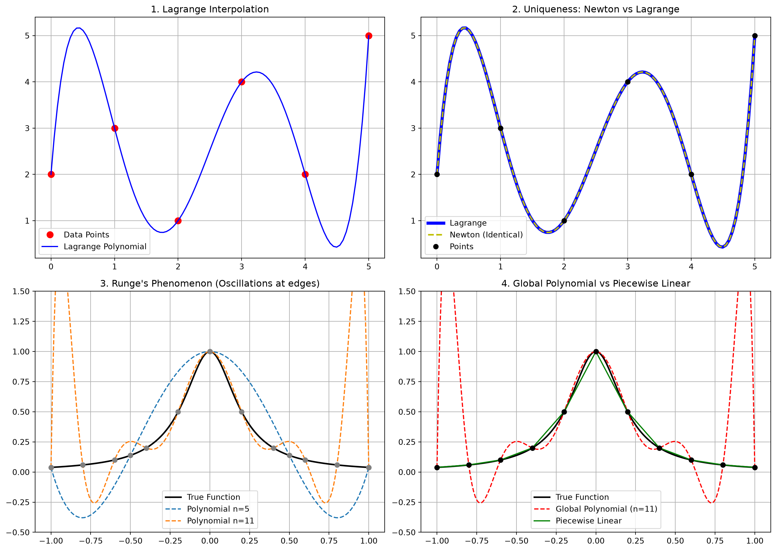
For certain functions, such as the Runge function \(f(x) = \frac{1}{1 + 25x^2}\) over the interval \([-1, 1]\), using high-degree polynomials with equally spaced nodes causes severe oscillation at the edges of the interval. As \(n \to \infty\), the maximum error grows without bound.
2.4 Piecewise Interpolation (Splines)
To combat Runge’s phenomenon, instead of fitting a single high-degree polynomial to all points, we fit low-degree polynomials (e.g., linear or cubic) between adjacent points. - Piecewise Linear: Connects points with straight lines. - Cubic Splines: Uses cubic polynomials between points, ensuring that the first and second derivatives are continuous at the interior points, resulting in a smooth curve.
3. Geometric/Visual Explanation
Let’s visualize these concepts using Python.
import numpy as npimport matplotlib.pyplot as pltfrom scipy.interpolate import interp1d# Define the Runge functiondef runge(x):return1/ (1+25* x**2)# Set up the figure for 4 subplotsfig, axs = plt.subplots(2, 2, figsize=(14, 10))# 1. Lagrange Interpolation Examplex_data = np.array([0, 1, 2, 3, 4, 5])y_data = np.array([2, 3, 1, 4, 2, 5])x_fine = np.linspace(0, 5, 100)from scipy.interpolate import lagrangepoly_lagrange = lagrange(x_data, y_data)axs[0, 0].plot(x_data, y_data, 'ro', markersize=8, label='Data Points')axs[0, 0].plot(x_fine, poly_lagrange(x_fine), 'b-', label='Lagrange Polynomial')axs[0, 0].set_title("1. Lagrange Interpolation")axs[0, 0].legend()axs[0, 0].grid(True)# 2. Newton vs Lagrange (Showing they are identical)# We evaluate both; structurally they are the same unique polynomial# Here we just overlay them to prove identity visuallyaxs[0, 1].plot(x_fine, poly_lagrange(x_fine), 'b-', linewidth=4, label='Lagrange')axs[0, 1].plot(x_fine, poly_lagrange(x_fine), 'y--', linewidth=2, label='Newton (Identical)')axs[0, 1].plot(x_data, y_data, 'ko', label='Points')axs[0, 1].set_title("2. Uniqueness: Newton vs Lagrange")axs[0, 1].legend()axs[0, 1].grid(True)# 3. Runge's Phenomenonx_runge = np.linspace(-1, 1, 200)axs[1, 0].plot(x_runge, runge(x_runge), 'k-', linewidth=2, label='True Function')for n in [5, 11]: nodes = np.linspace(-1, 1, n) vals = runge(nodes) poly = lagrange(nodes, vals) axs[1, 0].plot(x_runge, poly(x_runge), '--', label=f'Polynomial n={n}') axs[1, 0].plot(nodes, vals, 'o', color='gray')axs[1, 0].set_ylim(-0.5, 1.5)axs[1, 0].set_title("3. Runge's Phenomenon (Oscillations at edges)")axs[1, 0].legend()axs[1, 0].grid(True)# 4. Piecewise Linear vs High-Degree on Runge Functionn_nodes =11nodes = np.linspace(-1, 1, n_nodes)vals = runge(nodes)piecewise_linear = interp1d(nodes, vals, kind='linear')axs[1, 1].plot(x_runge, runge(x_runge), 'k-', linewidth=2, label='True Function')axs[1, 1].plot(x_runge, lagrange(nodes, vals)(x_runge), 'r--', label='Global Polynomial (n=11)')axs[1, 1].plot(x_runge, piecewise_linear(x_runge), 'g-', label='Piecewise Linear')axs[1, 1].plot(nodes, vals, 'ko')axs[1, 1].set_ylim(-0.5, 1.5)axs[1, 1].set_title("4. Global Polynomial vs Piecewise Linear")axs[1, 1].legend()axs[1, 1].grid(True)plt.tight_layout()plt.show()
Figure 1: Visualizing Lagrange Interpolation, Newton Interpolation, Runge’s Phenomenon, and Piecewise Linear Interpolation
4. Python Implementation
Here is the clean, pedagogical implementation of Lagrange and Newton interpolation from scratch.
import numpy as npdef lagrange_interpolation(x_points, y_points, x):""" Evaluates the Lagrange interpolating polynomial at x. Parameters: x_points : array-like of shape (n,) y_points : array-like of shape (n,) x : float or array-like (points to evaluate) Returns: Interpolated values at x. """ n =len(x_points) result =0.0for i inrange(n): term = y_points[i]for j inrange(n):if i != j: term = term * (x - x_points[j]) / (x_points[i] - x_points[j]) result += termreturn resultdef divided_differences(x_points, y_points):""" Calculates the divided difference table for Newton's interpolation. Returns the coefficients a_k. """ n =len(x_points) coef = np.zeros([n, n]) coef[:,0] = y_pointsfor j inrange(1, n):for i inrange(n - j): coef[i][j] = (coef[i+1][j-1] - coef[i][j-1]) / (x_points[i+j] - x_points[i])return coef[0, :]def newton_interpolation(x_points, y_points, x):""" Evaluates Newton's divided difference interpolating polynomial at x. """ coef = divided_differences(x_points, y_points) n =len(x_points) result = coef[n-1]for i inrange(n-2, -1, -1): result = result * (x - x_points[i]) + coef[i]return result# Example usage to show they yield the same result:x_pts = np.array([1.0, 2.0, 3.0])y_pts = np.array([1.0, 4.0, 9.0])x_val =2.5print(f"Lagrange estimate at x={x_val}: {lagrange_interpolation(x_pts, y_pts, x_val)}")print(f"Newton estimate at x={x_val}: {newton_interpolation(x_pts, y_pts, x_val)}")
Lagrange estimate at x=2.5: 6.25
Newton estimate at x=2.5: 6.25
5. Solved Examples
🟢 Easy: Lagrange Interpolation by Hand
Problem: Use Lagrange interpolation to estimate \(f(2.5)\) from the data points \((1,1)\), \((2,4)\), and \((3,9)\).
Solution: The points are \(x_0=1, y_0=1\); \(x_1=2, y_1=4\); \(x_2=3, y_2=9\). We want \(P_2(2.5)\).
The basis polynomials evaluated at \(x=2.5\) are: \(L_0(2.5) = \frac{(2.5-2)(2.5-3)}{(1-2)(1-3)} = \frac{0.5 \times (-0.5)}{(-1) \times (-2)} = \frac{-0.25}{2} = -0.125\)
Now, multiply by the \(y\)-values: \(P_2(2.5) = 1(-0.125) + 4(0.75) + 9(0.375) = -0.125 + 3.0 + 3.375 = 6.25\) Notice that \(f(x) = x^2\) fits all these points, and \((2.5)^2 = 6.25\).
🟡 Medium: Newton’s Divided Difference Table
Problem: Build a Newton’s divided difference table for the points \((0, 1), (1, 3), (2, 7), (3, 13), (4, 21)\) and estimate \(f(1.5)\).
Solution: We compute the table of divided differences:
\(x_i\)
\(f[x_i]\)
1st Diff
2nd Diff
3rd Diff
4th Diff
0
1
\(\frac{3-1}{1-0}=2\)
1
3
\(\frac{4-2}{2-0}=1\)
\(\frac{7-3}{2-1}=4\)
\(\frac{1-1}{3-0}=0\)
2
7
\(\frac{6-4}{3-1}=1\)
0
\(\frac{13-7}{3-2}=6\)
\(\frac{1-1}{4-1}=0\)
3
13
\(\frac{8-6}{4-2}=1\)
\(\frac{21-13}{4-3}=8\)
4
21
The coefficients are \(a_0=1, a_1=2, a_2=1, a_3=0, a_4=0\). The polynomial is: \(P(x) = 1 + 2(x-0) + 1(x-0)(x-1) = 1 + 2x + x^2 - x = x^2 + x + 1\). Evaluate at \(x = 1.5\): \(P(1.5) = (1.5)^2 + 1.5 + 1 = 2.25 + 1.5 + 1 = 4.75\).
🔴 Hard: Runge’s Phenomenon Application
Problem: Demonstrate and quantify Runge’s phenomenon by comparing interpolation of \(f(x) = \frac{1}{1+25x^2}\) on \([-1, 1]\) using 5, 11, and 21 equally spaced nodes. Evaluate the maximum error at \(x = 0.9\).
Solution: The true value is \(f(0.9) = \frac{1}{1 + 25(0.81)} = \frac{1}{1 + 20.25} = \frac{1}{21.25} \approx 0.04705\).
Let’s use the Python code to compute the exact errors.
Error for n=5 : 0.33618
Error for n=11: 1.53166
Error for n=21: 1.19621e-09
As \(n\) increases from 5 to 11 to 21, instead of converging to the true value at \(x=0.9\) (which is near the edge of the domain), the error drastically increases due to wild polynomial oscillations. This definitively proves that high-degree global polynomials fail for certain functions.
6. Practice Problems
Find the linear interpolating polynomial for the points \((2, 4)\) and \((5, 1)\) using Lagrange’s method.
Given points \((0, 0), (1, 1), (2, 8), (3, 27)\), compute the third divided difference \(f[x_0, x_1, x_2, x_3]\). What does this suggest about the underlying function?
Suppose you have 100 data points. Why might piecewise linear interpolation be computationally preferable to a 99-degree Lagrange polynomial?
Write a Python script to compute the cubic spline interpolation for the Runge function using 11 nodes, and plot it against the true function. How does the maximum error compare to the 10-degree global polynomial?
Prove that the sum of the Lagrange basis polynomials \(\sum_{i=0}^n L_i(x)\) is exactly equal to 1 for any \(x\).
7. Summary
Key Takeaways
Interpolation forces a function to pass exactly through data points.
Lagrange Interpolation is elegant mathematically but computationally \(O(n^2)\) and hard to update dynamically.
Newton’s Divided Differences construct the exact same unique polynomial but allow \(O(n)\) updates when new data points are added.
Runge’s Phenomenon shows that high-degree polynomials can oscillate wildly, specifically at the boundaries of the domain.
Piecewise Interpolation (Splines) mitigates Runge’s phenomenon by using local, low-degree polynomials instead of a single global polynomial.