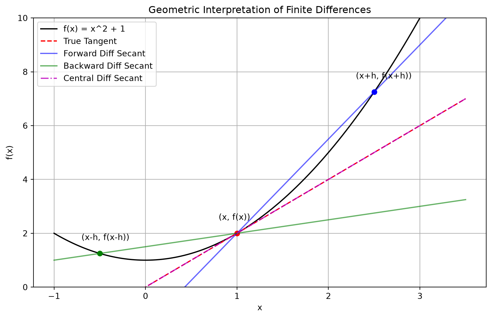
Numerical differentiation is the process of estimating the derivative of a mathematical function using values of the function. In many real-world physics and engineering applications, an analytical expression for a function may not be available. Instead, we might only have discrete data points from an experiment or simulation, such as position measurements over time, from which we need to derive velocity and acceleration. Alternatively, the function might be known but analytically intractable to differentiate. Numerical differentiation provides robust methods for approximating these derivatives and understanding the intrinsic trade-offs between mathematical truncation errors and computational round-off errors.
2. Theory
The foundation of most numerical differentiation formulas is the Taylor series expansion. For a sufficiently smooth function \(f(x)\), its value near a point \(x\) can be expanded as:
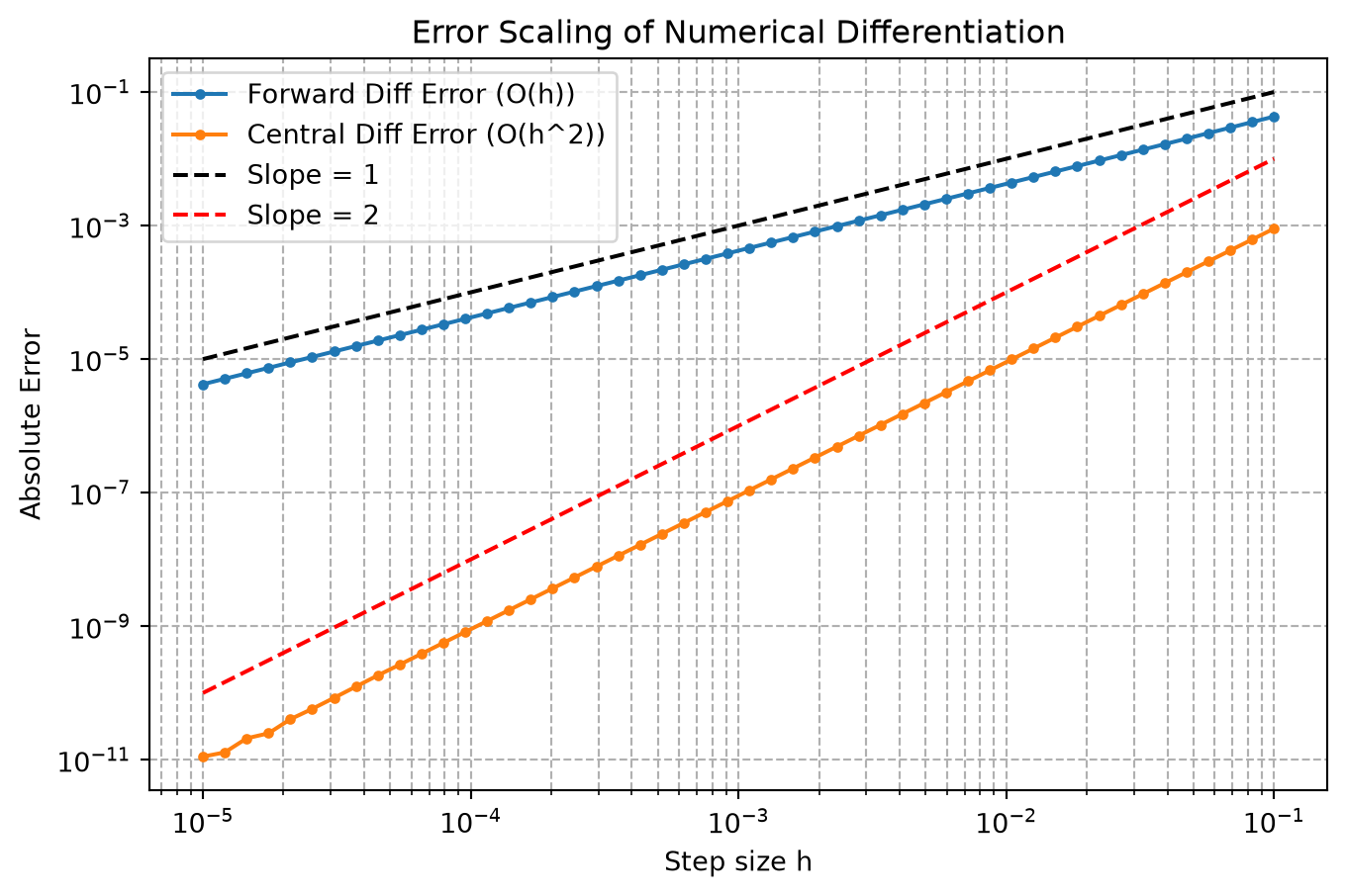
The leading error term is proportional to \(h\), so we say this method is \(\mathcal{O}(h)\) accurate.
Backward Difference
Similarly, using the expansion for \(f(x-h)\): \[f(x-h) = f(x) - hf'(x) + \frac{h^2}{2!}f''(x) - \frac{h^3}{3!}f'''(x) + \mathcal{O}(h^4)\]\[f'(x) \approx \frac{f(x) - f(x-h)}{h}\] This is also an \(\mathcal{O}(h)\) approximation.
Central Difference
If we subtract the \(f(x-h)\) expansion from the \(f(x+h)\) expansion, the even terms cancel out: \[f(x+h) - f(x-h) = 2hf'(x) + \frac{2h^3}{3!}f'''(x) + \dots\]\[f'(x) \approx \frac{f(x+h) - f(x-h)}{2h}\] The leading error term is proportional to \(h^2\), making the central difference an \(\mathcal{O}(h^2)\) method, which is significantly more accurate than forward or backward differences for small \(h\).
Higher-Order Derivatives
To find the second derivative, we can add the Taylor expansions for \(f(x+h)\) and \(f(x-h)\): \[f(x+h) + f(x-h) = 2f(x) + h^2 f''(x) + \mathcal{O}(h^4)\]\[f''(x) \approx \frac{f(x+h) - 2f(x) + f(x-h)}{h^2}\] This is an \(\mathcal{O}(h^2)\) approximation for the second derivative.
Richardson Extrapolation
Richardson extrapolation is a technique to improve the accuracy of a numerical approximation. If we have an \(\mathcal{O}(h^2)\) central difference estimate \(D(h)\) for \(f'(x)\): \[D(h) = f'(x) + c_1 h^2 + c_2 h^4 + \dots\] Evaluating with a step size of \(h/2\): \[D(h/2) = f'(x) + c_1 (h/2)^2 + c_2 (h/2)^4 + \dots = f'(x) + \frac{c_1}{4} h^2 + \frac{c_2}{16} h^4 + \dots\] We can eliminate the \(h^2\) error term by computing: \[D_{\text{ext}} = \frac{4D(h/2) - D(h)}{3}\] This new estimate is \(\mathcal{O}(h^4)\) accurate.
Optimal Step Size: Truncation vs. Round-off Error
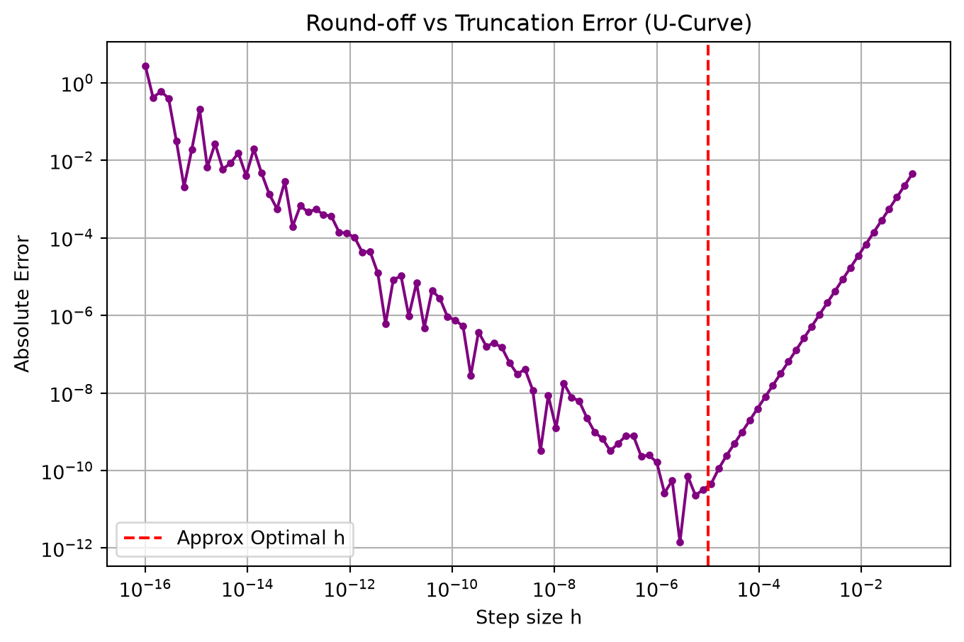
When computing numerically, decreasing \(h\) reduces the mathematical truncation error (the terms ignored in the Taylor series). However, as \(h \to 0\), \(f(x+h)\) and \(f(x)\) become nearly equal, leading to subtractive cancellation (a form of round-off error in floating-point arithmetic). Dividing by a very small \(h\) amplifies this round-off error. The total error is approximately \(E(h) = \frac{\epsilon}{h} + c h^n\), where \(\epsilon\) is machine precision. There exists an optimal step size \(h_{\text{opt}}\) that minimizes this total error.
Figure 2: Log-log plot of truncation errors for Forward vs Central Differences.
4. Python Implementation
import numpy as npdef forward_difference(f, x, h=1e-5):"""Computes the forward difference approximation of f'(x)."""return (f(x + h) - f(x)) / hdef backward_difference(f, x, h=1e-5):"""Computes the backward difference approximation of f'(x)."""return (f(x) - f(x - h)) / hdef central_difference(f, x, h=1e-5):"""Computes the central difference approximation of f'(x)."""return (f(x + h) - f(x - h)) / (2* h)def second_derivative(f, x, h=1e-5):"""Computes the central difference approximation of f''(x)."""return (f(x + h) -2* f(x) + f(x - h)) / (h**2)def richardson_extrapolation(f, x, h=1e-1):"""Improves the central difference estimate using Richardson Extrapolation.""" D_h = central_difference(f, x, h) D_h_half = central_difference(f, x, h /2)return (4* D_h_half - D_h) /3
5. Solved Examples
🟢 Easy: Finite Differences for \(f(x) = x^3\)
Problem: Compute the forward, backward, and central difference approximations of \(f'(1)\) for \(f(x) = x^3\) using \(h=0.1\). Compare with the exact value.
Solution: The exact derivative is \(f'(x) = 3x^2\), so \(f'(1) = 3(1)^2 = 3\). Given \(h=0.1\): \(f(1) = 1^3 = 1\)\(f(1.1) = 1.1^3 = 1.331\)\(f(0.9) = 0.9^3 = 0.729\)
🟡 Medium: Richardson Extrapolation for \(\cos(x)\)
Problem: Use Richardson Extrapolation to improve a central difference estimate of the derivative of \(f(x) = \cos(x)\) at \(x = \pi/4\), starting with \(h = 0.2\).
Actually, \(D(0.1)\) is closer to exact, the extrapolation yields: \(D_{\text{ext}} = \frac{4D(0.1) - D(0.2)}{3} \approx \frac{4(-0.7041785) - (-0.704545)}{3} \approx -0.704056...\)\(D_{\text{ext}}\) will yield an \(\mathcal{O}(h^4)\) approximation, matching the true value to more decimal places.
🔴 Hard: The Optimal Step Size for \(e^x\)
Problem: Compute the central difference derivative of \(f(x) = e^x\) at \(x=1\) for \(h\) ranging from \(10^{-1}\) down to \(10^{-16}\). Plot the error and find the optimal step size \(h_{\text{opt}}\).
Figure 3: Trade-off between truncation error and round-off error.
The plot clearly demonstrates the “U-curve”. As \(h\) decreases from \(10^{-1}\), the error drops because the mathematical truncation error \(\mathcal{O}(h^2)\) decreases. However, around \(h = 10^{-5}\), the error hits a minimum. For \(h < 10^{-5}\), the error rapidly increases due to the round-off error dominating the subtractive cancellation in floating-point arithmetic.
6. Practice Problems
Find the forward, backward, and central difference approximations for the derivative of \(f(x) = \ln(x)\) at \(x=2\) with \(h=0.1\).
Derive the \(\mathcal{O}(h^2)\) forward difference formula for the first derivative using Taylor series expansions for \(f(x+h)\) and \(f(x+2h)\).
The central difference formula for the second derivative is given in the text. Determine its leading error term order by substituting the Taylor series for \(f(x+h)\) and \(f(x-h)\).
Apply Richardson Extrapolation twice (to eliminate \(h^2\) and \(h^4\) terms) starting with central differences for \(f(x) = \sin(x)\) at \(x=\pi/3\) using \(h=0.4, 0.2, 0.1\).
A student attempts to calculate the derivative of a very noisy experimental dataset using the central difference method. What problems will they encounter, and why might they need to use a curve-fitting method (like least squares) before differentiating?
Richardson Extrapolation: A technique to boost the order of accuracy of an approximation method (e.g., from \(\mathcal{O}(h^2)\) to \(\mathcal{O}(h^4)\)).
Optimal Step Size (\(h\)): We must balance mathematical truncation error (requires small \(h\)) and computational round-off error (requires sufficiently large \(h\)). For central difference, optimal \(h \approx \sqrt[3]{\epsilon}\), where \(\epsilon\) is machine precision.