Module 8: Numerical Integration

Introduction

Numerical integration, often called quadrature, is the process of approximating the definite integral of a function: \[ I = \int_a^b f(x) dx \] In physics and engineering, integration is required to calculate work done by a variable force, center of mass, total charge, magnetic flux, and probabilities. When analytical integration is impossible or the function is only known at discrete data points, numerical methods are essential.

Theory

1. Newton-Cotes Formulas

Newton-Cotes formulas approximate the integrand \(f(x)\) with a polynomial of degree \(n\) that passes through equally spaced points, and then integrate the polynomial exactly.

Rectangle and Midpoint Methods (Degree 0)

Approximates the area as a series of rectangles. - Left Rectangle: \(I \approx \sum f(x_i) \Delta x\) - Midpoint: \(I \approx \sum f(\frac{x_i + x_{i+1}}{2}) \Delta x\)

Trapezoidal Rule (Degree 1)

Approximates the function with a straight line between \(a\) and \(b\). \[ \int_a^b f(x) dx \approx (b - a) \frac{f(a) + f(b)}{2} \] Composite Trapezoidal Rule: Divide \([a,b]\) into \(n\) segments of width \(h = \frac{b-a}{n}\). \[ I \approx \frac{h}{2} \left[ f(x_0) + 2 \sum_{i=1}^{n-1} f(x_i) + f(x_n) \right] \] Error: \(O(h^2)\).

Simpson’s 1/3 Rule (Degree 2)

Approximates the function using a parabola passing through 3 points. \[ \int_a^b f(x) dx \approx \frac{b-a}{6} \left[ f(a) + 4f\left(\frac{a+b}{2}\right) + f(b) \right] \] Composite Simpson’s 1/3 Rule: (Requires an even number of segments \(n\)) \[ I \approx \frac{h}{3} \left[ f(x_0) + 4\sum_{i=1,3,5}^{n-1} f(x_i) + 2\sum_{j=2,4,6}^{n-2} f(x_j) + f(x_n) \right] \] Error: \(O(h^4)\). Significantly more accurate than trapezoidal.

Simpson’s 3/8 Rule (Degree 3)

Uses a cubic polynomial through 4 points. Useful when the number of segments is a multiple of 3. \[ I \approx \frac{3h}{8} [f(x_0) + 3f(x_1) + 3f(x_2) + f(x_3)] \]

2. Gauss Quadrature

Newton-Cotes formulas use equally spaced points. Gauss Quadrature optimizes both the weights and the locations of the evaluation points (nodes) to achieve the highest possible accuracy for a given number of points. An \(n\)-point Gaussian quadrature rule integrates polynomials of degree up to \(2n-1\) exactly. \[ \int_{-1}^1 f(x) dx \approx \sum_{i=1}^n w_i f(x_i) \] Where \(x_i\) are the roots of Legendre polynomials, and \(w_i\) are specific weights. For a general interval \([a,b]\), a coordinate transformation is applied: \(x = \frac{b-a}{2}t + \frac{b+a}{2}\).

Geometric / Visual Explanation

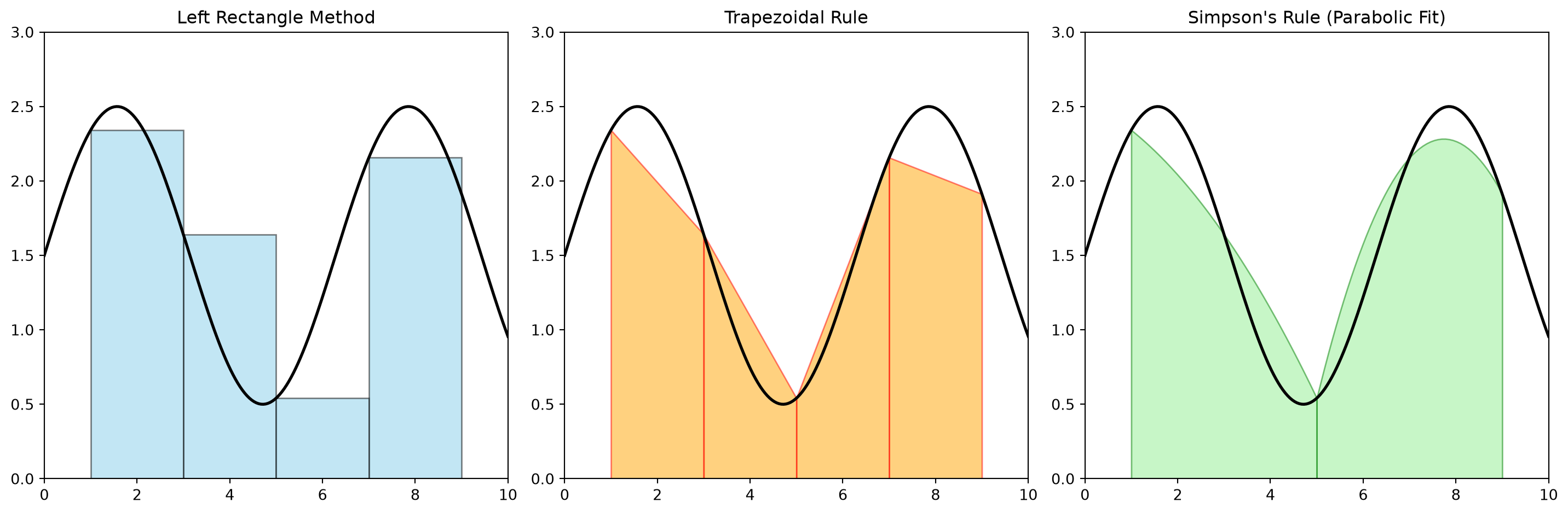
Let’s visualize how these methods approximate the area under a curve.

import numpy as np
import matplotlib.pyplot as plt

def f(x): return np.sin(x) + 1.5

x = np.linspace(0, 10, 200)
y = f(x)
a, b = 1, 9
n = 4
x_trap = np.linspace(a, b, n+1)
y_trap = f(x_trap)

plt.figure(figsize=(15, 5))

# 1. Left Rectangle
plt.subplot(1, 3, 1)
plt.plot(x, y, 'k-', lw=2)
for i in range(n):
    plt.gca().add_patch(plt.Rectangle((x_trap[i], 0), x_trap[i+1]-x_trap[i], y_trap[i], 
                                      facecolor='skyblue', edgecolor='black', alpha=0.5))
plt.title("Left Rectangle Method")
plt.xlim(0, 10); plt.ylim(0, 3)

# 2. Trapezoidal
plt.subplot(1, 3, 2)
plt.plot(x, y, 'k-', lw=2)
for i in range(n):
    plt.fill_between([x_trap[i], x_trap[i+1]], [0, 0], [y_trap[i], y_trap[i+1]], 
                     color='orange', edgecolor='red', alpha=0.5)
plt.title("Trapezoidal Rule")
plt.xlim(0, 10); plt.ylim(0, 3)

# 3. Simpson's (Parabolas)
plt.subplot(1, 3, 3)
plt.plot(x, y, 'k-', lw=2)
x_simp = np.linspace(a, b, 2) # n=2 for visual simplicity
for i in range(0, len(x_trap)-2, 2):
    xs = np.linspace(x_trap[i], x_trap[i+2], 50)
    coeffs = np.polyfit([x_trap[i], x_trap[i+1], x_trap[i+2]], 
                        [y_trap[i], y_trap[i+1], y_trap[i+2]], 2)
    ys = np.polyval(coeffs, xs)
    plt.fill_between(xs, 0, ys, color='lightgreen', edgecolor='green', alpha=0.5)
plt.title("Simpson's Rule (Parabolic Fit)")
plt.xlim(0, 10); plt.ylim(0, 3)

plt.tight_layout()
plt.show()

Python Implementation

import numpy as np

def trapezoidal(f, a, b, n):
    h = (b - a) / n
    x = np.linspace(a, b, n+1)
    y = f(x)
    return (h/2) * (y[0] + 2*np.sum(y[1:-1]) + y[-1])

def simpson13(f, a, b, n):
    if n % 2 != 0:
        raise ValueError("n must be even for Simpson's 1/3 rule")
    h = (b - a) / n
    x = np.linspace(a, b, n+1)
    y = f(x)
    return (h/3) * (y[0] + 4*np.sum(y[1:-1:2]) + 2*np.sum(y[2:-2:2]) + y[-1])

def gauss_quadrature_2pt(f, a, b):
    # Transformation
    def transform(t):
        return ((b-a)*t + a+b)/2.0
    
    # 2-point nodes and weights
    t1, t2 = -1/np.sqrt(3), 1/np.sqrt(3)
    w1, w2 = 1.0, 1.0
    
    integral = w1 * f(transform(t1)) + w2 * f(transform(t2))
    return integral * (b-a)/2.0

Solved Examples

🟢 Easy: Trapezoidal Rule

Problem: Compute \(\int_0^2 x^2 dx\) using the trapezoidal rule with \(n=4\). Solution: \(h = \frac{2-0}{4} = 0.5\). Points: \(x = [0, 0.5, 1.0, 1.5, 2.0]\). Values: \(y = [0, 0.25, 1.0, 2.25, 4.0]\). \(I \approx \frac{0.5}{2} [0 + 2(0.25 + 1.0 + 2.25) + 4.0] = 0.25 [0 + 7.0 + 4.0] = 0.25 \times 11 = 2.75\). (Exact is \(8/3 \approx 2.667\)).

🟡 Medium: Simpson’s Rule

Problem: Compute \(\int_0^\pi \sin(x) dx\) using Simpson’s 1/3 rule with \(n=6\). Solution: \(h = \pi/6\). \(I \approx \frac{\pi/18}{3} [ \sin(0) + 4(\sin(\pi/6) + \sin(3\pi/6) + \sin(5\pi/6)) + 2(\sin(2\pi/6) + \sin(4\pi/6)) + \sin(\pi) ]\). \(I \approx \frac{\pi}{18} [ 0 + 4(0.5 + 1 + 0.5) + 2(0.866 + 0.866) + 0 ] \approx 2.00086\). (Exact is 2.0).

🔴 Hard: Gauss Quadrature vs Trapezoidal

Problem: Compare Trapezoidal (\(n=2\)) and 2-point Gauss Quadrature on \(\int_0^1 e^{-x^2} dx\). Solution: Trapezoidal (\(n=2, h=0.5\)): \(I_T = \frac{0.5}{2}[1 + 2(e^{-0.25}) + e^{-1}] \approx 0.25[1 + 1.5576 + 0.3678] \approx 0.731\). Gauss (2-point): Transform \(t\) to \(x\): \(x = 0.5t + 0.5\). \(I_G = 0.5 [ e^{-(0.5(-1/\sqrt{3})+0.5)^2} + e^{-(0.5(1/\sqrt{3})+0.5)^2} ] \approx 0.7468\). (Exact is \(\approx 0.746824\)). Gauss quadrature is astoundingly more accurate for the same number of evaluations!

Practice Problems

Compute \(\int_1^3 \frac{1}{x} dx\) using the Midpoint rule with \(n=4\).
Derive the error bound formula for the Composite Trapezoidal Rule.
Why does Simpson’s 1/3 rule require an even number of intervals?
Write a Python function for 3-point Gauss Quadrature.
Compare the convergence rates of Trapezoidal and Simpson’s methods as \(n \to \infty\).

Summary

Key Formulas

Trapezoidal Rule (\(O(h^2)\)): \(I \approx \frac{h}{2}[f_0 + 2\sum f_i + f_n]\)
Simpson’s 1/3 Rule (\(O(h^4)\)): \(I \approx \frac{h}{3}[f_0 + 4\sum_{odd} f_i + 2\sum_{even} f_i + f_n]\)
Gauss Quadrature: Uses optimal roots of Legendre polynomials to maximize polynomial exactness. Extremely efficient.

← Back to Course Index