In physics and engineering, the laws of nature are most naturally expressed as relationships between changing quantities. These relationships are formalized mathematically as Differential Equations. Whether calculating the trajectory of a spacecraft, analyzing the decay of radioactive isotopes, or modeling the dynamics of an electrical circuit, Ordinary Differential Equations (ODEs) play a foundational role.
While exact analytical solutions exist for linear and some simple non-linear ODEs, the vast majority of physical systems—especially those involving non-linear dynamics, chaos, or complex interactions—cannot be solved exactly. In these cases, numerical methods are indispensable for finding approximate solutions.
Theory
Initial Value Problems (IVPs)
A first-order ordinary differential equation can generally be written in the form: \[ \frac{dy}{dt} = f(t, y) \] where \(y\) is the state variable, \(t\) is the independent variable (often time), and \(f(t, y)\) is a known function describing the rate of change of \(y\).
An Initial Value Problem (IVP) specifies the state of the system at some starting time \(t_0\): \[ y(t_0) = y_0 \] Our goal is to compute \(y(t)\) for \(t > t_0\) by taking discrete steps of size \(h\). Let \(t_n = t_0 + n h\). We seek approximations \(y_n \approx y(t_n)\).
Euler’s Method (Forward Euler)
The simplest numerical method is Euler’s Method. We can derive it using the Taylor series expansion of \(y(t)\) around \(t_n\): \[ y(t_{n+1}) = y(t_n + h) = y(t_n) + h y'(t_n) + \frac{h^2}{2} y''(t_n) + \dots \] Truncating after the linear term and substituting \(y'(t_n) = f(t_n, y_n)\) gives: \[ y_{n+1} = y_n + h f(t_n, y_n) \]
Error: The local truncation error (error made in a single step) is \(O(h^2)\), but over \(N \propto 1/h\) steps, the global error accumulates to \(O(h)\). Hence, Euler’s method is a first-order method.
Modified/Improved Euler Method (Heun’s Method)
Euler’s method uses the derivative at the beginning of the interval to step across the entire interval, which can lead to large errors if the slope changes rapidly. Heun’s method improves this using a predictor-corrector approach: 1. Predictor: Compute an intermediate guess using standard Euler: \[ \tilde{y}_{n+1} = y_n + h f(t_n, y_n) \] 2. Corrector: Average the slopes at the start and the predicted end of the interval: \[ y_{n+1} = y_n + \frac{h}{2} \left[ f(t_n, y_n) + f(t_{n+1}, \tilde{y}_{n+1}) \right] \] This is a second-order method with a global error of \(O(h^2)\).
Runge-Kutta Methods
Runge-Kutta (RK) methods evaluate the derivative \(f(t,y)\) at several stages within the interval \([t_n, t_{n+1}]\) and combine them to achieve higher-order accuracy without needing higher derivatives of \(f\).
RK2 (Midpoint Method)
This is another second-order method: \[ k_1 = h f(t_n, y_n) \]\[ k_2 = h f\left(t_n + \frac{h}{2}, y_n + \frac{k_1}{2}\right) \]\[ y_{n+1} = y_n + k_2 \]
RK4 (Classical Fourth-Order)
The RK4 method is the workhorse of numerical ODE solvers. It uses four stages and achieves \(O(h^4)\) global accuracy. \[ k_1 = h f(t_n, y_n) \]\[ k_2 = h f\left(t_n + \frac{h}{2}, y_n + \frac{k_1}{2}\right) \]\[ k_3 = h f\left(t_n + \frac{h}{2}, y_n + \frac{k_2}{2}\right) \]\[ k_4 = h f(t_n + h, y_n + k_3) \]\[ y_{n+1} = y_n + \frac{1}{6}(k_1 + 2k_2 + 2k_3 + k_4) \]
Systems of ODEs
Higher-order ODEs can be converted into systems of first-order ODEs. For example, Newton’s second law \(\frac{d^2x}{dt^2} = F(x, v, t)/m\) becomes: \[ \frac{dx}{dt} = v \]\[ \frac{dv}{dt} = \frac{1}{m}F(x, v, t) \] Vectorizing the state \(\mathbf{y} = [x, v]^T\), we can apply methods like RK4 directly: \(\mathbf{y}_{n+1} = \mathbf{y}_n + \frac{1}{6}(\mathbf{k}_1 + 2\mathbf{k}_2 + 2\mathbf{k}_3 + \mathbf{k}_4)\).
Boundary Value Problems (BVPs): Shooting Method
Unlike IVPs, Boundary Value Problems (BVPs) specify conditions at two different points (e.g., \(y(a) = \alpha\), \(y(b) = \beta\)). The Shooting Method converts a BVP into an IVP by guessing the missing initial condition (e.g., \(y'(a)\)), integrating to \(b\), and adjusting the guess iteratively (using a root-finding algorithm like Secant or Newton’s method) until \(y(b) = \beta\) is satisfied.
Stability and Stiff Equations
An ODE is considered stiff if some components of the solution vary much more rapidly than others, forcing the solver to take extremely small step sizes to maintain stability (even if the rapid transient has already died out). Explicit methods (like forward Euler or RK4) struggle with stiffness. Implicit methods (like Backward Euler: \(y_{n+1} = y_n + h f(t_{n+1}, y_{n+1})\)) are typically required for stiff equations due to their larger stability regions.
Geometric / Visual Explanation
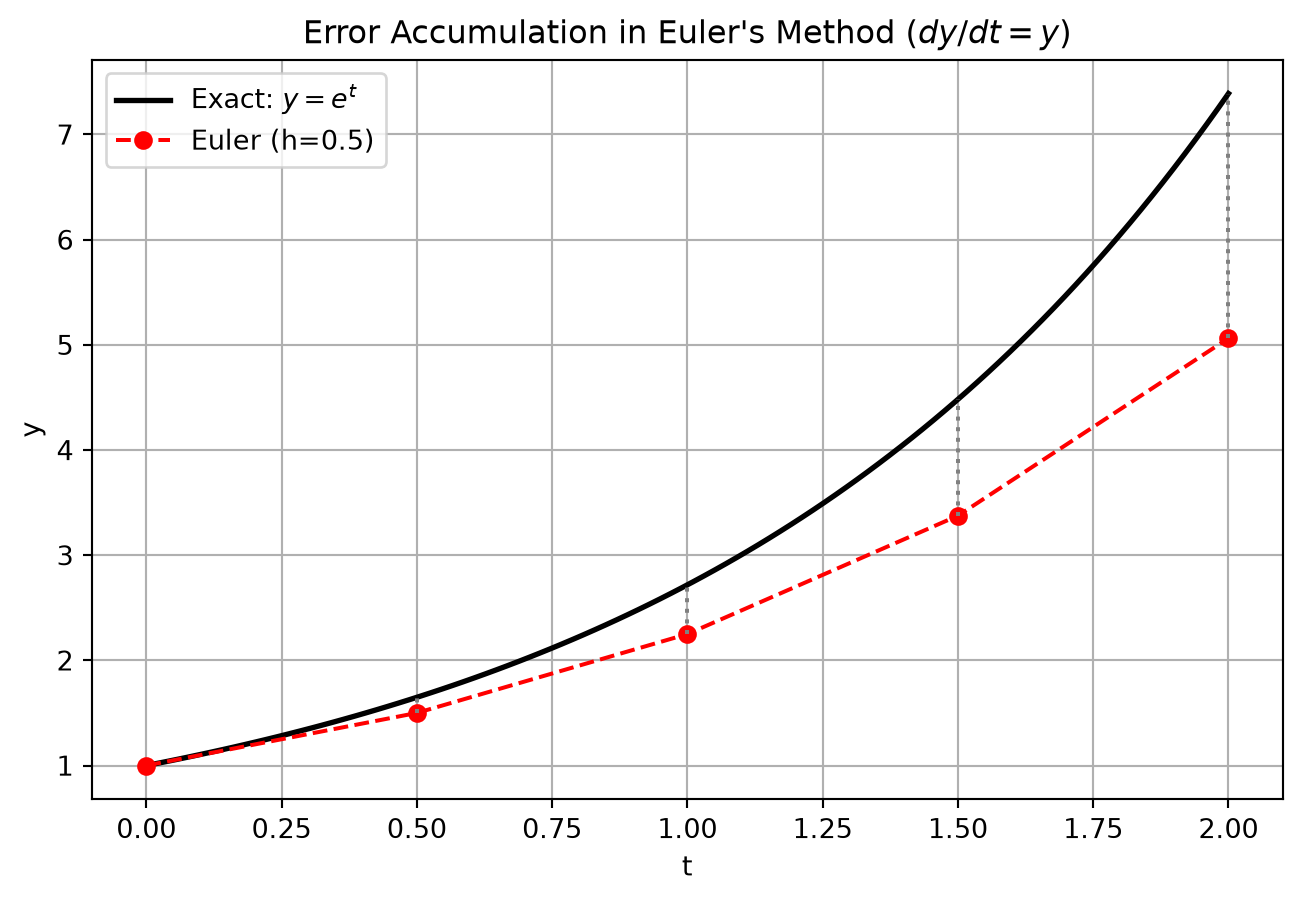
import numpy as npimport matplotlib.pyplot as pltdef exact_sol(t):return np.exp(t)t_exact = np.linspace(0, 2, 100)y_exact = exact_sol(t_exact)h =0.5t_euler = np.arange(0, 2.1, h)y_euler = np.zeros(len(t_euler))y_euler[0] =1.0for i inrange(len(t_euler)-1): y_euler[i+1] = y_euler[i] + h * y_euler[i]plt.figure(figsize=(8,5))plt.plot(t_exact, y_exact, label="Exact: $y = e^t$", color='black', linewidth=2)plt.plot(t_euler, y_euler, 'o--', label=f"Euler (h={h})", color='red')for i inrange(len(t_euler)): plt.vlines(t_euler[i], y_euler[i], exact_sol(t_euler[i]), color='gray', linestyle=':')plt.title("Error Accumulation in Euler's Method ($dy/dt = y$)")plt.xlabel("t")plt.ylabel("y")plt.legend()plt.grid(True)plt.show()
Figure 1: Euler’s method accumulates error rapidly compared to the exact solution.
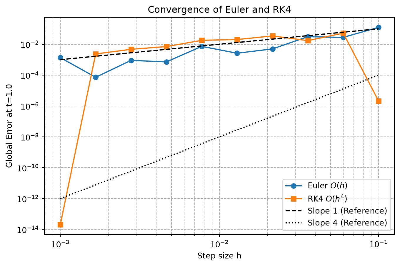
Figure 4: Convergence Plot: Global Error vs Step Size (h) for Euler and RK4.
Python Implementation
Below is a robust object-oriented implementation of the RK4 method capable of handling both scalar ODEs and systems of ODEs.
import numpy as npdef rk4_step(f, t, y, h):""" Takes a single Runge-Kutta 4th order step. Parameters: f : callable The derivative function f(t, y). Must handle vector y if solving a system. t : float Current time. y : float or numpy.ndarray Current state. h : float Step size. Returns: numpy.ndarray Next state. """ k1 = h * f(t, y) k2 = h * f(t +0.5*h, y +0.5*k1) k3 = h * f(t +0.5*h, y +0.5*k2) k4 = h * f(t + h, y + k3)return y + (k1 +2*k2 +2*k3 + k4) /6.0def solve_ode(f, t_span, y0, h):""" Solves an IVP using RK4. Parameters: f : callable f(t, y) t_span : tuple (t_start, t_end) y0 : float or numpy.ndarray Initial condition. h : float Step size. """ t_start, t_end = t_span t_eval = np.arange(t_start, t_end + h, h)# Handle both scalar and vector systems y0 = np.asarray(y0)if y0.ndim ==0: y_eval = np.zeros(len(t_eval))else: y_eval = np.zeros((len(t_eval), len(y0))) y_eval[0] = y0for i inrange(len(t_eval) -1): y_eval[i+1] = rk4_step(f, t_eval[i], y_eval[i], h)return t_eval, y_eval
Solved Examples
🟢 Easy: Euler’s Method by Hand
Problem: Solve \(\frac{dy}{dt} = -2y\) with \(y(0)=1\) using Euler’s method for 5 steps with \(h=0.1\).
Problem: Solve the same ODE \(\frac{dy}{dt} = -2y\) using RK4 with \(h=0.1\) for one step and compare with the exact solution.
Solution: Start at \(t=0, y=1\). - \(k_1 = h f(t, y) = 0.1 \times (-2 \times 1) = -0.2\) - \(k_2 = h f(t + h/2, y + k_1/2) = 0.1 \times (-2 \times (1 - 0.1)) = -0.18\) - \(k_3 = h f(t + h/2, y + k_2/2) = 0.1 \times (-2 \times (1 - 0.09)) = -0.182\) - \(k_4 = h f(t + h, y + k_3) = 0.1 \times (-2 \times (1 - 0.182)) = -0.1636\)
\(y_1 = 1 + \frac{1}{6}(-0.2 + 2(-0.18) + 2(-0.182) + (-0.1636)) = 1 - 0.181266 = 0.818733\) Exact is \(e^{-0.2} \approx 0.818730\). The error is on the order of \(10^{-6}\)!
🔴 Hard: Damped Harmonic Oscillator (System of ODEs)
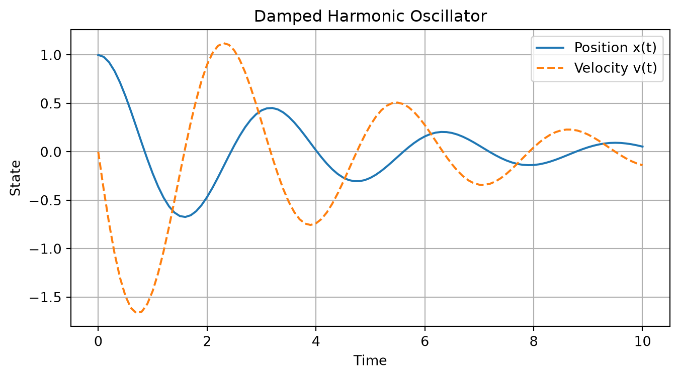
Problem: Solve \(x'' + 0.5x' + 4x = 0\) with \(x(0)=1, x'(0)=0\) up to \(t=10\) using RK4.
Solution: Define \(y_1 = x\) and \(y_2 = x'\). The system is: \(y_1' = y_2\)\(y_2' = -4y_1 - 0.5y_2\)
Euler’s Method: Apply Euler’s method to solve \(y' = t - y\) with \(y(0)=1\) for \(t \in [0, 0.5]\) using \(h=0.1\).
Heun’s Method: Solve the same problem using Heun’s (Improved Euler) method and compare the result at \(t=0.5\) to the exact solution \(y(t) = t - 1 + 2e^{-t}\).
RK4 Application: Use RK4 with \(h=0.2\) to solve the non-linear ODE \(y' = y^2 + 1\) with \(y(0)=0\) for one step. Check your answer against the exact solution \(y = \tan(t)\).
Systems Setup: Convert the non-linear pendulum equation \(\theta'' + \frac{g}{L} \sin(\theta) = 0\) into a system of two first-order ODEs.
Shooting Method Logic: Describe the steps required to solve the BVP \(y'' = -y, y(0)=0, y(\pi/2)=1\) using the Shooting Method and Euler integration. What root-finding equation are you trying to satisfy?
Summary
Key Takeaways and Formulas
Initial Value Problems (IVPs) require numerical integration to step forward in time from a known initial state.
Runge-Kutta 4 (\(O(h^4)\)):\[ y_{n+1} = y_n + \frac{1}{6}(k_1 + 2k_2 + 2k_3 + k_4) \] where \(k\) terms sample the derivative at various points in the interval.
Higher-order ODEs must be converted into systems of first-order ODEs before standard numerical solvers can be applied.