Partial Differential Equations (PDEs) form the backbone of theoretical physics and engineering. While Ordinary Differential Equations (ODEs) describe systems with a single independent variable (usually time), PDEs deal with functions of multiple independent variables, typically spatial coordinates and time.
Almost every fundamental physical law is expressed as a PDE: - Heat Transfer: How temperature evolves in a material over time. - Electrostatics: The electric potential distribution in space due to charge configurations. - Fluid Dynamics: The Navier-Stokes equations governing the flow of fluids. - Quantum Mechanics: The Schrödinger equation describing wavefunctions. - Vibrations: The motion of a vibrating string or drumhead.
Because analytical solutions to PDEs are only available for highly symmetric and simplified geometries, numerical methods are absolutely essential for solving real-world physical problems.
2. Theory
2.1 Classification of PDEs
Second-order linear PDEs in two variables \((x, y)\) take the general form: \[ A \frac{\partial^2 u}{\partial x^2} + B \frac{\partial^2 u}{\partial x \partial y} + C \frac{\partial^2 u}{\partial y^2} + D \frac{\partial u}{\partial x} + E \frac{\partial u}{\partial y} + F u = G \]
The equation is classified by the discriminant \(\Delta = B^2 - 4AC\):
Elliptic (\(\Delta < 0\)): e.g., Laplace’s Equation \(\nabla^2 u = 0\). Describes steady-state equilibrium phenomena (e.g., electrostatics, steady temperature). Information propagates instantly in all directions.
Hyperbolic (\(\Delta > 0\)): e.g., Wave Equation \(\frac{\partial^2 u}{\partial t^2} = c^2 \nabla^2 u\). Describes wave propagation. Information travels at a finite speed \(c\).
2.2 Finite Difference Method for PDEs
The Finite Difference Method (FDM) replaces continuous partial derivatives with discrete difference approximations on a grid. We define a spatial grid \(x_i = i \Delta x\), \(y_j = j \Delta y\), and time steps \(t_n = n \Delta t\). We denote the numerical approximation of \(u(x_i, y_j, t_n)\) as \(u_{i,j}^n\).
Using Taylor series expansions, the second derivatives in space are approximated as: \[ \frac{\partial^2 u}{\partial x^2} \approx \frac{u_{i+1,j} - 2u_{i,j} + u_{i-1,j}}{(\Delta x)^2} \]
2.3 Laplace’s Equation (Elliptic)
The 2D Laplace’s equation for a steady-state quantity (like electric potential or steady temperature) is: \[ \frac{\partial^2 u}{\partial x^2} + \frac{\partial^2 u}{\partial y^2} = 0 \]
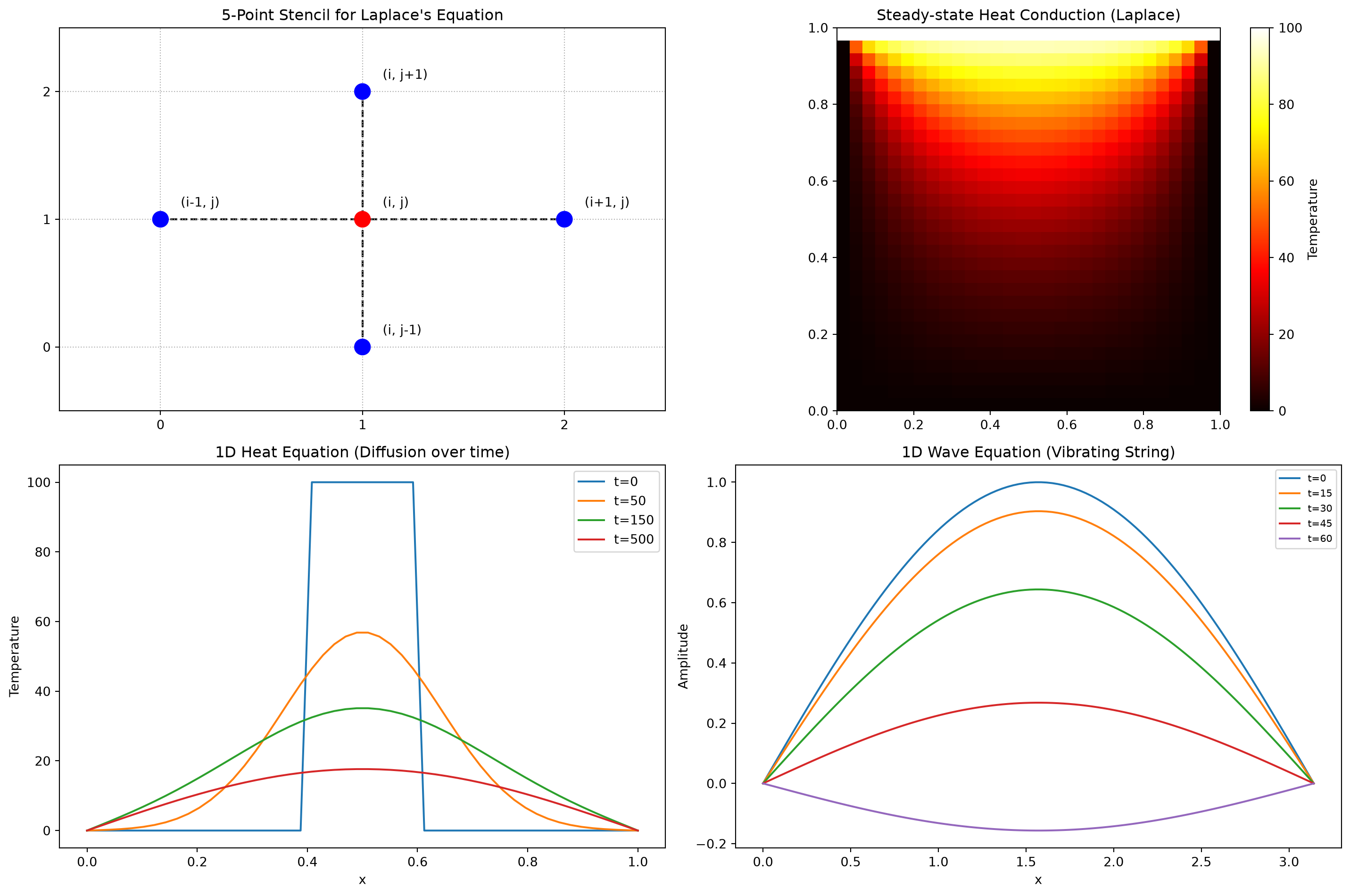
Assuming \(\Delta x = \Delta y = h\), substituting the finite difference approximations yields the 5-point stencil: \[ \frac{u_{i+1,j} - 2u_{i,j} + u_{i-1,j}}{h^2} + \frac{u_{i,j+1} - 2u_{i,j} + u_{i,j-1}}{h^2} = 0 \]\[ u_{i,j} = \frac{1}{4} (u_{i+1,j} + u_{i-1,j} + u_{i,j+1} + u_{i,j-1}) \] This states that the value at any point is the average of its four nearest neighbors. We can solve this system of linear equations iteratively using methods like Jacobi or Gauss-Seidel.
2.4 Heat Equation (Parabolic)
The 1D Heat Equation is: \[ \frac{\partial u}{\partial t} = \alpha \frac{\partial^2 u}{\partial x^2} \] where \(\alpha\) is the thermal diffusivity.
Using a forward difference in time and central difference in space (FTCS - Forward Time Centered Space): \[ \frac{u_i^{n+1} - u_i^n}{\Delta t} = \alpha \frac{u_{i+1}^n - 2u_i^n + u_{i-1}^n}{(\Delta x)^2} \] Solving for the future state \(u_i^{n+1}\): \[ u_i^{n+1} = u_i^n + r (u_{i+1}^n - 2u_i^n + u_{i-1}^n) \] where \(r = \frac{\alpha \Delta t}{(\Delta x)^2}\). For this explicit scheme to be numerically stable, it must satisfy the CFL (Courant-Friedrichs-Lewy) stability condition: \(r \le 0.5\).
2.5 Wave Equation (Hyperbolic)
The 1D Wave Equation describes a vibrating string: \[ \frac{\partial^2 u}{\partial t^2} = c^2 \frac{\partial^2 u}{\partial x^2} \] Using central differences for both time and space: \[ \frac{u_i^{n+1} - 2u_i^n + u_i^{n-1}}{(\Delta t)^2} = c^2 \frac{u_{i+1}^n - 2u_i^n + u_{i-1}^n}{(\Delta x)^2} \] Solving for the future position \(u_i^{n+1}\): \[ u_i^{n+1} = 2u_i^n - u_i^{n-1} + C^2 (u_{i+1}^n - 2u_i^n + u_{i-1}^n) \] where \(C = \frac{c \Delta t}{\Delta x}\) is the Courant number. For stability, we require \(C \le 1\).
Figure 1: Visualizing the components and solutions of PDEs
4. Python Implementation
Here is a clean implementation of the 1D Heat Equation solver using the explicit FTCS scheme.
import numpy as npimport matplotlib.pyplot as pltdef solve_heat_equation_1d(L, T, nx, nt, alpha, initial_cond):""" Solves the 1D Heat Equation u_t = alpha * u_xx using FTCS. Parameters: L : Length of the spatial domain [0, L] T : Total time of simulation [0, T] nx : Number of spatial grid points nt : Number of time steps alpha: Thermal diffusivity initial_cond: Function evaluating the initial condition u(x, 0) Returns: x_grid : Spatial grid points u : Final temperature distribution at time T """ dx = L / (nx -1) dt = T / nt r = alpha * dt / (dx**2)if r >0.5:print(f"Warning: r = {r:.3f} > 0.5. The solution may be unstable!") x_grid = np.linspace(0, L, nx) u = initial_cond(x_grid) u_new = np.zeros_like(u)for n inrange(nt):# Update interior pointsfor i inrange(1, nx -1): u_new[i] = u[i] + r * (u[i+1] -2*u[i] + u[i-1])# Apply Dirichlet boundary conditions (fixed to 0) u_new[0] =0.0 u_new[-1] =0.0# Move to next time step u[:] = u_new[:]return x_grid, u
5. Solved Examples
🟢 Easy: Grid Setup for Laplace’s Equation
Problem: Set up the system of equations for Laplace’s equation on a \(4 \times 4\) grid (\(0 \le i, j \le 3\)). The boundaries are: \(u(0,j) = 0\), \(u(3,j) = 100\), \(u(i,0) = 0\), \(u(i,3) = 100\).
Solution: A \(4 \times 4\) grid means indices \(i, j \in \{0, 1, 2, 3\}\). The interior points are only those where \(i \in \{1, 2\}\) and \(j \in \{1, 2\}\). So we have exactly 4 interior unknowns: \(u_{1,1}, u_{2,1}, u_{1,2}, u_{2,2}\).
This forms a simple \(4 \times 4\) linear system that can be solved directly or iteratively!
🟡 Medium: Solving the 1D Heat Equation
Problem: A metal rod of length \(L=1\) m has an initial temperature \(u(x,0) = \sin(\pi x)\) (in °C). Its ends are kept at 0°C. The thermal diffusivity is \(\alpha = 0.01\). Find the temperature distribution at \(t=0.5\)s using \(\Delta x = 0.1\) and \(\Delta t = 0.1\).
Solution: 1. Check stability: \(r = \frac{\alpha \Delta t}{(\Delta x)^2} = \frac{0.01 \times 0.1}{(0.1)^2} = \frac{0.001}{0.01} = 0.1\). Since \(r \le 0.5\), the FTCS scheme is stable. 2. Grid setup: \(x_i = i \times 0.1\) for \(i = 0, ..., 10\). 3. At \(t=0\), \(u_i^0 = \sin(0.1 \pi i)\). 4. Applying FTCS for the first time step \(t=0.1\): \[ u_i^1 = u_i^0 + 0.1(u_{i+1}^0 - 2u_i^0 + u_{i-1}^0) \] For instance, at \(i=1\) (\(x=0.1\)): \(u_1^0 = \sin(0.1\pi) \approx 0.3090\)\(u_0^0 = 0\)\(u_2^0 = \sin(0.2\pi) \approx 0.5878\)\(u_1^1 = 0.3090 + 0.1(0.5878 - 2(0.3090) + 0) = 0.3090 - 0.0030 = 0.3060\) °C. We repeat this for 5 time steps to reach \(t=0.5\)s.
🔴 Hard: Laplace’s Equation via Gauss-Seidel Iteration
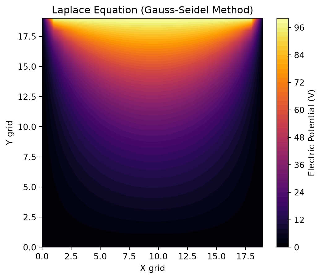
Problem: Solve Laplace’s equation on a \(20 \times 20\) grid using Gauss-Seidel iteration. The top edge is held at 100V, while the left, right, and bottom edges are at 0V. Visualize the result.
Solution: Unlike the Jacobi method which uses old values for all updates, Gauss-Seidel uses the newly updated values immediately, which accelerates convergence.
Classification: Classify the following PDE: \(3\frac{\partial^2 u}{\partial x^2} - 2\frac{\partial^2 u}{\partial x \partial y} + 4\frac{\partial^2 u}{\partial y^2} = 0\).
Stability: For the 1D Heat Equation with \(\alpha = 0.5\) m\(^2\)/s and \(\Delta x = 0.05\) m, what is the maximum allowable time step \(\Delta t\) for the FTCS scheme to be stable?
Difference Equations: Derive the explicit finite difference update rule for the 1D Advection Equation \(\frac{\partial u}{\partial t} + v \frac{\partial u}{\partial x} = 0\) using forward difference in time and backward difference in space.
Wave Equation: Given a string discretized with \(\Delta x = 0.1\), \(c = 2.0\). If \(\Delta t = 0.02\), calculate the position of node \(i\) at step \(n+1\) if \(u_i^n = 1.0\), \(u_i^{n-1} = 0.8\), \(u_{i+1}^n = 1.2\), \(u_{i-1}^n = 1.2\).
Programming: Modify the provided solve_heat_equation_1d python function to use Neumann boundary conditions (insulating ends where \(\frac{\partial u}{\partial x} = 0\)) instead of Dirichlet boundary conditions.
7. Summary
Module 10 Summary
Key Takeaways: - PDE Classification: Second-order linear PDEs are Elliptic (\(B^2-4AC < 0\)), Parabolic (\(B^2-4AC = 0\)), or Hyperbolic (\(B^2-4AC > 0\)). - Finite Difference Method: Translates continuous derivatives into discrete algebraic equations using Taylor series approximations. - Laplace’s Equation (Elliptic): Modeled using the 5-point stencil \(u_{i,j} = \frac{1}{4}(u_{i+1,j} + \dots)\). Solved iteratively (Jacobi/Gauss-Seidel). - Heat Equation (Parabolic): Modeled using FTCS. Conditionally stable: requires \(r = \frac{\alpha \Delta t}{\Delta x^2} \le 0.5\). - Wave Equation (Hyperbolic): Models wave propagation. Conditionally stable: requires Courant number \(C = \frac{c \Delta t}{\Delta x} \le 1\).