In the natural sciences and engineering, we frequently encounter periodic phenomena—from the vibration of atoms in a crystal lattice to the orbits of planets, the propagation of electromagnetic waves, and the transmission of acoustic signals. While analyzing these phenomena in the time domain (as a function of time) is intuitive, it often obscures the underlying physics.
Fourier Analysis is the mathematical framework that allows us to transition from the time domain to the frequency domain. By decomposing a complex signal into a sum of simple sinusoidal waves of different frequencies, we can easily identify the dominant vibrational modes, filter out unwanted noise, and solve complex differential equations that govern wave mechanics and heat transfer. Fourier approximation is arguably one of the most important numerical tools in modern computational physics.
Theory
Fourier Series
For a continuous, periodic function \(f(t)\) with period \(T\), the Fourier Series representation is given by an infinite sum of sines and cosines:
\[ f(t) = \frac{a_0}{2} + \sum_{n=1}^{\infty} \left( a_n \cos(2\pi n f_0 t) + b_n \sin(2\pi n f_0 t) \right) \]
where \(f_0 = 1/T\) is the fundamental frequency, and the coefficients are given by: \[ a_n = \frac{2}{T} \int_{0}^{T} f(t) \cos(2\pi n f_0 t) \, dt, \quad b_n = \frac{2}{T} \int_{0}^{T} f(t) \sin(2\pi n f_0 t) \, dt \]
Alternatively, using Euler’s formula \(e^{i\theta} = \cos\theta + i\sin\theta\), we can write the complex Fourier series: \[ f(t) = \sum_{n=-\infty}^{\infty} c_n e^{i 2\pi n f_0 t} \]\[ c_n = \frac{1}{T} \int_{0}^{T} f(t) e^{-i 2\pi n f_0 t} \, dt \]
Discrete Fourier Transform (DFT)
In computational physics, signals are rarely continuous. Instead, they are sampled at discrete time intervals. Suppose we have \(N\) uniformly spaced samples of a signal, \(y_k = f(t_k)\) for \(k = 0, 1, \dots, N-1\), with a sampling interval \(\Delta t\).
The Discrete Fourier Transform (DFT) converts this discrete time-domain signal into a discrete frequency-domain spectrum. The DFT is defined as:
\[ Y_k = \sum_{n=0}^{N-1} y_n e^{-i 2\pi k n / N} \] for \(k = 0, 1, \dots, N-1\). The coefficients \(Y_k\) represent the amplitude and phase of the various frequency components.
The inverse DFT is given by: \[ y_n = \frac{1}{N} \sum_{k=0}^{N-1} Y_k e^{i 2\pi k n / N} \]
Nyquist Frequency and Aliasing
When sampling a signal, the highest frequency that can be accurately resolved without ambiguity is the Nyquist frequency, defined as half the sampling rate: \[ f_{Nyquist} = \frac{1}{2\Delta t} \] If the signal contains frequencies higher than the Nyquist frequency, they will “fold back” and appear as lower-frequency artifacts. This phenomenon is known as aliasing.
Fast Fourier Transform (FFT)
Computing the DFT directly requires on the order of \(O(N^2)\) operations, which becomes prohibitively slow for large datasets (e.g., millions of points). The Fast Fourier Transform (FFT) algorithm, popularized by Cooley and Tukey in 1965, exploits the periodic properties of the complex exponential to reduce the computational complexity to \(O(N \log N)\). This revolutionary algorithm makes real-time signal processing and large-scale spectral analysis feasible.
Power Spectral Density (PSD)
To quantify the power or energy of each frequency component, we compute the Power Spectral Density: \[ P_k = \frac{|Y_k|^2}{N} \] The PSD highlights the dominant frequencies that contribute most significantly to the total variance of the signal.
Geometric and Visual Explanation
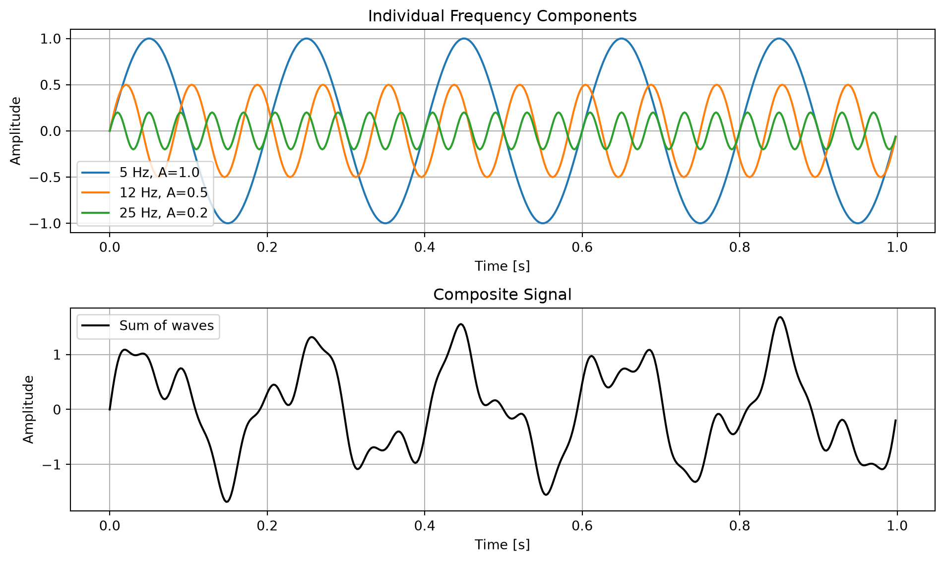
Let’s visualize the core concept: building a complex signal from simple sines, and then using the FFT to extract those frequencies.
import numpy as npimport matplotlib.pyplot as plt# Time arrayt = np.linspace(0, 1, 500, endpoint=False)# Three different sine wavesf1, f2, f3 =5, 12, 25# Frequencies in HzA1, A2, A3 =1.0, 0.5, 0.2# Amplitudesy1 = A1 * np.sin(2* np.pi * f1 * t)y2 = A2 * np.sin(2* np.pi * f2 * t)y3 = A3 * np.sin(2* np.pi * f3 * t)# Composite signaly_sum = y1 + y2 + y3fig, (ax1, ax2) = plt.subplots(2, 1, figsize=(10, 6))ax1.plot(t, y1, label=f'{f1} Hz, A={A1}')ax1.plot(t, y2, label=f'{f2} Hz, A={A2}')ax1.plot(t, y3, label=f'{f3} Hz, A={A3}')ax1.set_title('Individual Frequency Components')ax1.set_xlabel('Time [s]')ax1.set_ylabel('Amplitude')ax1.legend()ax1.grid(True)ax2.plot(t, y_sum, color='black', label='Sum of waves')ax2.set_title('Composite Signal')ax2.set_xlabel('Time [s]')ax2.set_ylabel('Amplitude')ax2.legend()ax2.grid(True)plt.tight_layout()plt.show()
Figure 1: Top: Individual sine waves. Bottom: The composite signal constructed by summing them.
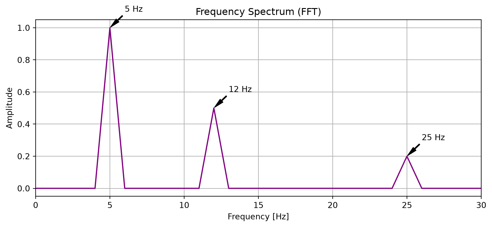
Now, we compute the FFT of this composite signal to see the frequency spectrum.
from scipy.fft import fft, fftfreqN =len(t)dt = t[1] - t[0]# Compute FFTyf = fft(y_sum)# Compute frequency binsxf = fftfreq(N, dt)[:N//2] # Keep only positive frequencies# Magnitude of the FFT# Normalize by 2/N to get true amplitudesmagnitude =2.0/N * np.abs(yf[0:N//2])plt.figure(figsize=(10, 4))plt.plot(xf, magnitude, color='purple')plt.title('Frequency Spectrum (FFT)')plt.xlabel('Frequency [Hz]')plt.ylabel('Amplitude')plt.grid(True)plt.xlim(0, 30)# Annotate peaksfor f, A inzip([f1, f2, f3], [A1, A2, A3]): plt.annotate(f'{f} Hz', xy=(f, A), xytext=(f+1, A+0.1), arrowprops=dict(facecolor='black', shrink=0.05, width=1, headwidth=5))plt.show()
Figure 2: FFT Frequency Spectrum of the composite signal showing distinct peaks at 5 Hz, 12 Hz, and 25 Hz.
Python Implementation
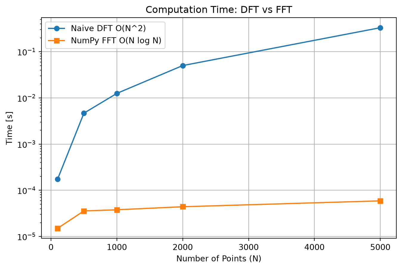
While numpy.fft or scipy.fft provide highly optimized FFT routines, it is instructive to see a naive DFT implementation to understand the mathematics. We can also compare the performance.
import timedef discrete_fourier_transform(y):""" Compute the 1D Discrete Fourier Transform naively. Time complexity: O(N^2) """ N =len(y) n = np.arange(N) k = n.reshape((N, 1))# Calculate the exponential matrix e = np.exp(-2j* np.pi * k * n / N)# Matrix multiplication to compute DFT Y = np.dot(e, y)return Y# Let's verify with a small arraysample_y = np.array([1.0, 2.0, 1.0, -1.0])print("Naive DFT:")print(np.round(discrete_fourier_transform(sample_y), 4))print("\\nNumPy FFT:")print(np.round(np.fft.fft(sample_y), 4))# Performance comparisonsizes = [100, 500, 1000, 2000, 5000]dft_times = []fft_times = []for s in sizes: test_y = np.random.random(s) start = time.time() _ = discrete_fourier_transform(test_y) dft_times.append(time.time() - start) start = time.time() _ = np.fft.fft(test_y) fft_times.append(time.time() - start)plt.figure(figsize=(8, 5))plt.plot(sizes, dft_times, marker='o', label='Naive DFT O(N^2)')plt.plot(sizes, fft_times, marker='s', label='NumPy FFT O(N log N)')plt.title('Computation Time: DFT vs FFT')plt.xlabel('Number of Points (N)')plt.ylabel('Time [s]')plt.legend()plt.grid(True)plt.yscale('log') # Log scale to show the stark differenceplt.show()
Figure 3: Comparison of computation time between naive DFT and optimized FFT as the number of data points increases.
Solved Examples
🟢 Easy: Hand calculation of DFT
Problem: Compute the DFT of the 4-point signal \(y = [1, 0, -1, 0]\).
Solution: We have \(N=4\). The DFT formula is \(Y_k = \sum_{n=0}^{3} y_n e^{-i 2\pi k n / 4} = \sum_{n=0}^{3} y_n e^{-i \pi k n / 2}\). Since \(y_1 = 0\) and \(y_3 = 0\), the sum simplifies to: \[ Y_k = y_0 e^0 + y_2 e^{-i \pi k} = 1 + (-1)(-1)^k = 1 - (-1)^k \]
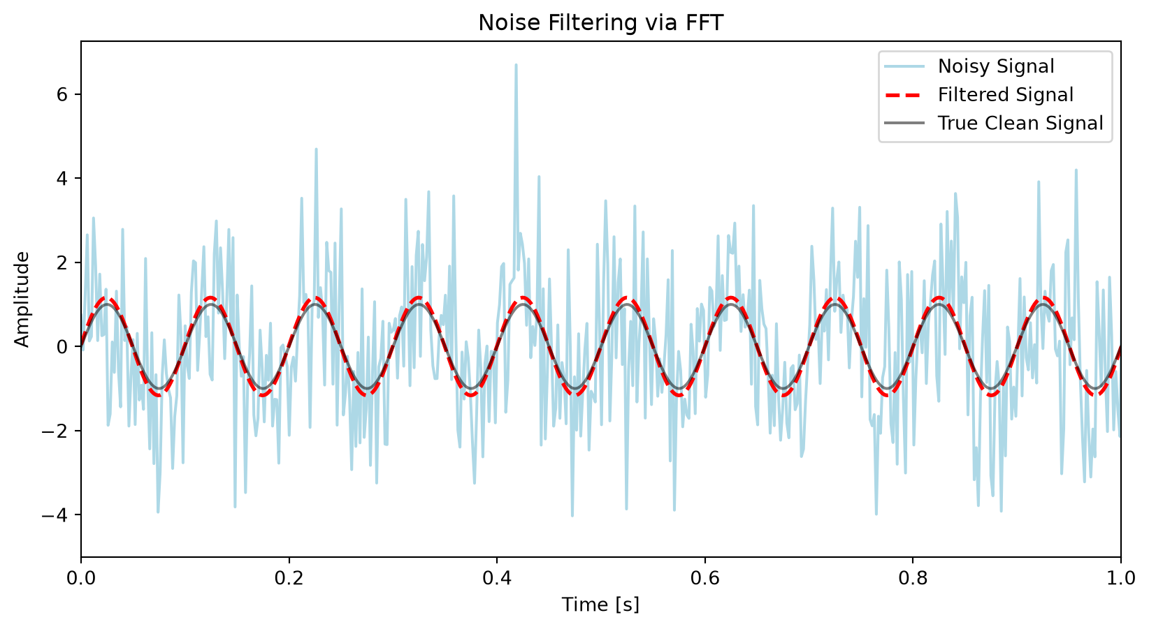
Problem: A 10 Hz signal is corrupted by high-frequency white noise. Use FFT to filter the noise by thresholding the frequency spectrum, then apply the Inverse FFT to recover the clean signal.
# 1. Create noisy signalt_noise = np.linspace(0, 2, 1000)clean_signal = np.sin(2* np.pi *10* t_noise)noise = np.random.normal(0, 1.5, 1000)noisy_signal = clean_signal + noise# 2. Compute FFTN_n =len(t_noise)yf_noisy = fft(noisy_signal)# 3. Filter in frequency domain (Power Spectral Density approach)# Calculate Power Spectral DensityPSD = (np.abs(yf_noisy) **2) / N_n# Find frequencies with large power (threshold = 100)indices = PSD >50# Zero out all small coefficients (filtering out noise)yf_clean = yf_noisy * indices# 4. Inverse FFT to get back to time domainrecovered_signal = np.fft.ifft(yf_clean).real# Plottingplt.figure(figsize=(10, 5))plt.plot(t_noise, noisy_signal, color='lightblue', label='Noisy Signal')plt.plot(t_noise, recovered_signal, color='red', linewidth=2, linestyle='--', label='Filtered Signal')plt.plot(t_noise, clean_signal, color='black', alpha=0.5, label='True Clean Signal')plt.title('Noise Filtering via FFT')plt.xlabel('Time [s]')plt.ylabel('Amplitude')plt.legend()plt.xlim(0, 1)plt.show()
Figure 4: Noise filtering using FFT: Original noisy signal (blue) and the recovered clean signal (red dashed).
Practice Problems
Nyquist Rate: You are sampling a signal containing frequencies up to \(500\) Hz. What is the absolute minimum sampling rate required to avoid aliasing? What sampling rate would you choose in practice?
Phase Retrieval: Modify the Python FFT code to plot the phase angle (np.angle) of the frequency components instead of just the magnitude. What does the phase tell you about the starting position of the sine waves?
DFT by hand: Compute the DFT of the sequence \(y = [2, 1, 2, 1]\) manually.
Square Wave Decomposition: Create a square wave signal in Python. Compute its FFT and plot the frequency spectrum. You should observe only odd harmonics. Verify that their amplitudes decay as \(1/n\).
Audio Filtering: Download a short .wav audio file (e.g., a bell ringing). Load it using scipy.io.wavfile. Apply an FFT, cut off all frequencies above \(2000\) Hz, perform an inverse FFT, and save it as a new .wav file. Listen to the difference.
Summary
Key Takeaways: Fourier Approximation
Time vs. Frequency: Fourier analysis transforms a signal from a function of time \(f(t)\) to a function of frequency \(F(\omega)\), revealing underlying oscillatory modes.
DFT: The Discrete Fourier Transform computes the frequency spectrum of a discretely sampled signal: \[ Y_k = \sum_{n=0}^{N-1} y_n e^{-i 2\pi k n / N} \]
FFT: The Fast Fourier Transform is an efficient algorithm that computes the DFT in \(O(N \log N)\) time, making real-time processing possible.
Nyquist Theorem: To accurately resolve a frequency \(f\), you must sample the signal at a rate of at least \(2f\).
Applications: Filtering noise by zeroing out specific frequency bins and performing the Inverse FFT (iFFT) is a cornerstone technique in digital signal processing.